Since the middle of the 20th century, ‘ecosystem’ has been a guiding scientific term for the pragmatic observation of ecological units (Jax 2016). An ecosystem encompasses the structure of relationships between living organisms and their inorganic environment. In a less abstract sense, an ecosystem is characterised by its biocoenosis and associated habitat (assemblage or community of plants and animals with the same or similar ecological demands in a distinct area) (Ellenberg et al. 1992). An ecological system is most frequently defined as “a community of organisms and their physical environment interacting as an ecological unit” (Lincoln et al. 1982). However, this structural view does not describe the substance of the term ‘ecosystem’, which primarily evolved to describe the functional relations inside ecosystems and within their network, thereby creating the biosphere of the earth (Vačkář et al. 2018). The term ‘biotope’ is almost synonymous with the term habitat, but while the subject of a habitat is a species or a population, the subject of a biotope is a biological community (Bastian et al. 2020).

Ecosystem research is a conceptual approach particularly identified by natural scientists, since it encompasses the creation of analytical models to examine the structure and dynamics of spatial regions (Grunewald and Bastian 2015). The ecosystem concept comprises several hierarchical levels, not only theoretically, but also from an operational point of view (Blasi et al. 2017). Therefore, in principle, a wide spatial-range of ecosystems can be identified and mapped on levels from biomes and ecoregions to habitats (EEA 2013, EEA 2014a, Klijn and de Haes 1994, Burkhard et al. 2018, Keith et al. 2020).

Ecosystems must be understood holistically. This means that their emergent system properties (interactions between their components) behave in a way that cannot be explained by simply analysing each individual component. Hence, we must attempt a holistic understanding, also in terms of our indicators and mappings. Furthermore, landscapes and ecosystems can be viewed, on the one hand, as the result of influential factors of the natural environment or, on the other hand, as a construct of human perception, i.e. as artificial units, whereby the criteria for the selection of the ecosystem components and their delimitation are determined by the particular interests of the observer (landscape as perceived by people). The Biodiversity Convention (CBD 2018) specifies the ecosystem approach as follows: “[…] the term ‘ecosystem’ […] can refer to any functioning unit at any scale. Indeed, the scale of analysis and action should be determined by the problem being addressed.”

For land cover mapping at the pan-European level, there exist established data sources such as Corine Land Cover (CLC), Land Use and Land Cover Survey (LUCAS) and the Farm Structure Survey (FSS). New high‑resolution Copernicus land‑monitoring products can increase the precision and relevance of these data (EEA 2017).

While land cover describes the physical material on the surface of the earth and its characteristics (e.g. grass, asphalt, trees bare ground, water etc.), land use is, by contrast, a description of how people use the land. Examples for land use are urban and agricultural land use, but also institutional land, sports grounds, residential land etc. (Fisher et al. 2005). In practice, ecosystem classifications are enhanced land cover maps and include additional information about abiotic and vegetation characteristics (EEA 2016; Burkhard et al. 2018). The Technical Recommendations in support of the SEEA‐EEA indicate that delineation of ecosystem assets (contiguous areas covered by a specific ecosystem) should be based on ecological and ecosystem use factors (UN - United Nation 2017). Ecosystem assets are the primary spatial units for ecosystem accounting (UN 2020).

When classifying ecosystems at national level for ecosystem accounting, EU member states are recommended to use the pan-European CORINE Land Cover (CLC) data on land use (Maes et al. 2014; Erhard et al. 2017). This regularly updated geo-dataset contains spatial information on land cover broken down into 44 classes. CORINE Land Cover data is provided for the years 1990, 2000, 2006, 2012 and 2018. The time series also includes a land-change layer, which highlights changes in land cover and land use. The spatial resolution is at least 25 ha. The European Nature Information System (EUNIS) offers a more detailed typology of ecosystems, taking into account the distribution of species and local spatial characteristics.

The general MAES typology of ecosystems (Maes et al. 2013) is organised into two levels. The first level is defined as “major ecosystem categories” and includes three main classes: 1) Terrestrial; 2) Fresh water; 3) Marine. At the second level, the major categories are subdivided into more detailed subclasses according to the character of their biophysical features. The terrestrial ecosystems are subdivided into seven subclasses: 1) Urban; 2) Cropland; 3) Grassland; 4) Woodland and forest; 5) Heathland and shrub; 6) Sparsely vegetated land; and 7) Wetlands. The fresh-water ecosystem class contains only one subclass, namely Rivers and lakes. Marine ecosystems are subdivided into four subclasses: 1) Marine inlets and transitional waters; 2) Coastal; 3) Shelf; and 4) Open ocean. Annex 2 of the MAES report (Maes et al. 2013) provides a table that links ecosystem types at level 2 with the CORINE Land Cover classification. Some ecosystem types fully correspond to an entire category of CORINE classes. For instance, urban ecosystems correspond to category 1. Artificial surfaces and include all classes from level one to three, while sparsely vegetated lands correspond to category 3.3 Open spaces with little or no vegetation. Other ecosystems correspond to classes from different levels of the CORINE classification. For instance, the ecosystem type grassland corresponds to categories 2.3.1 Pastures and 3.2.1 Natural grasslands, which are in different groups at level two of the CORINE classification (Nedkov et al. 2016).

The European Environmental Agency provides a dataset aimed at contributing to a better biological characterisation of terrestrial and marine ecosystems across Europe (EEA-39). It represents probabilities of the presence of EUNIS (European Nature Information System) habitats in terrestrial, freshwater and marine ecosystems. The work supports the Mapping and Assessment of Ecosystems and their Services (MAES), namely Action 5 in Target 2 of the EU Biodiversity Strategy to 2020, established to achieve the Aichi targets of the Convention on Biological Diversity (CBD). Input information and methods are documented in a technical paper (Weiss and Banko 2018).

With regard to the individual approaches of various EU countries in gathering the needed data, we can expect a differentiated picture. This will be outlined below by means of a few examples.

Estonia established a very short project of 18 months, creating a constraint in terms of time and workload (Helm and Prangel 2020). For this reason, it was necessary to prioritise ecosystem types, which was done by the Ministry of Environment, based on relevance for trans-sectoral policies. The following four ecosystems were selected: forest, grassland, agricultural/cropland and wetland. Each ecosystem was assessed by a team of experts, who also determined how to subdivide the ecosystem types, as follows:

• Forest: Subdivided according to the Estonian classification of site type groups (primarily based on soil type) to give 10 forest classes;
• Grassland: Initially subdivided according to soil management: Seeded, Permanent, Semi-natural. Semi-natural is further subdivided according to Annex I of the Estonian Habitat Code so that the results can be further “inserted” into the nature conservation policy;
• Agricultural/cropland: Subdivided according to soil fertility;
• Wetland: Subdivided according to soil type.

In Slovakia, a generalised nationwide map of ecosystems has been created using agricultural, forestry and environmental data (Černecký et al. 2020). The resulting polygons are classified as ecosystem/habitat types in accordance with the EUNIS classification system. The spatial precision of the data is determined by that of the field data, which was mostly created at scales of between 1:10,000 and 1:5,000. The data are stored in the form of a geo-database containing more than 1,000,000 polygons.

The work in Poland was divided into the following stages (Anonymous 2015):

1. Analysis of land cover forms defined according to CORINE Land Cover (CLC level 3) classification with respect to their occurrence on Polish territory;
2. A definition of types of ecosystems occurring in Poland, based on EUNIS ecosystem classification at levels 2 and 3;
3. Defining and delimitation of the basic assessment unit (BAU): basic typological unit representing a given ecosystem type (based on EUNIS classification) taking into account land cover features (according to CLC). The BAU is simultaneously the basic spatial operational unit for detailed analyses, including the assessment of ecosystem services based on thematic data.

The resolution of the database corresponds to scale 1:100,000. Minimal mapping units are:

• natural and semi-natural non-forested areas (meadows, pastures, wetlands, dunes and sands, sparsely vegetated areas) of size 10 ha;
• remaining areas (e.g. high-density buildings, industrial areas and transport networks, arable lands, forests) of size 25 ha;
• minimum width of the spatial unit: approx. 100 m.

In the Czech Republic, a more detailed map of the ecosystems, the so-called Consolidated Layer of Ecosystems of the Czech Republic (CLES), was developed in cooperation with the Czech Nature Conservation Agency. CLES presents a detailed map of the extent of natural, as well as artificial ecosystems in the national territory. It was developed by means of detailed habitat mapping in the Czech Republic, as well as by exploiting other data sources on agricultural land, urban areas and water bodies. The advantage of CLES is the detailed resolution of ecosystems down to the local level. However, in its current form, CLES cannot be used to track changes in the value of ecosystem services (Vačkář et al. 2018).

The Italian ecosystem types were identified and mapped by integrating the land cover database with additional spatial datasets that focus on biophysical features of the environment, such as bioclimate and vegetation (Blasi et al. 2017). Consistent with their spatial prevalence, the physiognomic CLC information was enhanced by means of the distinctive compositional, ecological and biogeographical features associated with each Potential Natural Vegetation (PNV). The Ecosystem Map of Italy consists of 84 types, comprising forests and semi-natural areas, wetlands and water bodies, out of a total of 97 legend classes, which also include artificial surfaces and agricultural areas. The typological correspondence with the second level of the EUNIS Habitat classification highlights the relationship, which is often hierarchical, between national ecosystem types and those recognised at the European level (Erhard et al. 2016).

The mapping of ecosystems in Bulgaria was based on CLC data and on MAES typology. Drawing on the CORINE dataset, nine main ecosystem types (according to MAES typology) can be delineated in Bulgaria. The scale of the output product was fixed at 1:100,000, giving a spatial precision of the CLC database of 100 m (N).

The following criteria were determined in developing the typology (classification) of ecosystems:

• clear and consistent classification principle (systematic organisation, cf. Burkhard et al. 2018; Grunewald et al. 2020);
• can be derived from existing data sources;
• compatible with international systems (such as MAES, EUNIS, cf. EEA 2016; IUCN, cf. Keith et al. 2020);
• classes can be illustrated in a spatially explicit manner in order to identify correlations with other locally-collected statistical data;
• data available for regular time periods (monitoring): changes in the various stocks/changes between classes (migration) quantifiable;
• current and future possibilities for incorporating nature conservation data available throughout Germany (Natura 2000 data, biotope mapping etc.);
• open for further development.

The European CLC classification system was used to define those ecosystem classes that, on the basis of the Digital Land Cover Model for Germany (Digitales Landbedeckungsmodell für Deutschland or LBM-DE), can be delimited with sufficient clarity. Of the 44 existing land cover classes for Europe, identified in the CLC nomenclature, 37 are relevant for Germany (Keil et al. 2015). An approach was developed to allow a redundancy-free description of all the land and marine areas under German jurisdiction by means of five main ETs, each of which encompasses three sub-types (or in the case of “forest and woodland”, two sub-ETs). This system also takes account of dynamic or complex ETs such as “transitional woodland/shrub” (CLC 3.2.4) (see Table 1).

Fig. 1 gives an overview of the proposed classification system. The core of the GIS-based monitoring of the ET areas is the system of CLC classes already defined for Germany. These can be aggregated into the levels of sub- or main ecosystem types. However, these CLC classes are not ideally suited for assessing the state of ecosystems with regard to nature conservation goals and, specifically, the protection of biodiversity. The requisite refinement of the system is indicated in Fig. 1 (right side) and explained in Section 3.4.

Figure 1.  

Schematic diagram of the proposed classification system for ecosystem types (ETs).

The proposed classificatory system has been aligned with the EUNIS classification (EUNIS 2019a) as far as possible with the utilised (land use) data. The 5,284 individual EUNIS habitat types (EUNIS 2019b) were grouped into the 10 main categories of the European ET map (plus habitat complexes), which include both terrestrial and marine types. For the individual habitat types, the EUNIS catalogue (EUNIS 2019a) defines correlations with other classification systems (including FFH types and the above-mentioned CLC classes). These have been largely adopted to enable the correct assignments to be made and thereby ensure a precise and consistent Europe-wide ecosystem accounting (EEA 2014b; Maes et al. 2014; Erhard et al. 2016). The relationship between the ETs and the EUNIS types can be found in Suppl. material 1 (Table A: Proposal of a classification system for ecosystem types (ETs) in Germany, assignment to the European ecosystem types according to EUNIS and to the CLC types of the database LBM-DE).

The aggregation of types required by the ET classification system takes account not only of the characteristics of land use and land cover, but also the rules of aggregation and the reliability of the data sources. The rules of aggregation state that small elements must be assigned to that ET of which they can be considered as spatial components (e.g. pastoral forests, hedges or bushes to the open land they are located in, springs to wetlands etc.). In order to keep the number of ETs manageable and to be able to work efficiently with the catalogue, land types that very rarely occur in Germany, which can change with great rapidity or are often recorded incorrectly by remote-sensing methods, were assigned to classes from which they sometimes differ to a large degree. This applies, for example, to glaciers (extremely rare), burnt areas (highly dynamic) or certain natural grassland types (rare and difficult to detect). For the sake of reliability, CLC classes that can hardly be distinguished from one another by analysing the base data, are grouped into relatively undifferentiated ETs, for example, coniferous, mixed and deciduous forests, as well as wooded dunes, are assigned to the class forest or wetlands, which also encompasses lowland moors (undetectable from space). Semantic ambiguity – such as the historically or technically controversial distinction between natural, fortified, straightened, diverted or canalised rivers and their (sometimes more natural but nevertheless artificially created) interconnected millraces and “real” canals – was also avoided in view of the small total extent of running waters. Ultimately, the relatively broad typology was chosen to avoid any unnecessary imprecision through the introduction of uncertainties inherent in finer classifications.

The specification of EU-wide approaches and data can be realised for Germany by means of the “Digital Basic Landscape Model” (Digitales Basis-Landschaftsmodell or Basis-DLM), derived from the “Official Topographic-Cartographic Information System” (ATKIS) and the “Digital Land Cover Model for Germany” (LBM-DE) (Schorcht et al. 2016), which represent the official National Spatial Data Infrastructure. The Basis-DLM contains “areas of actual use” (Flächen zur tatsächlichen Nutzung or TN) that are regularly monitored by the surveying authorities of the federal states of Germany in accordance with standard rules and with no spatial overlaps (Krüger et al. 2013; BKG 2016a). The LBM-DE for Germany is provided by the Federal Agency for Cartography and Geodesy (BKG), using classified satellite image data and the ATKIS-Basis-DLM, supplemented by other technical data. It is compatible with CLC data (and obeys the same nomenclature), but has a much more detailed scale of 1:50,000 (minimum mapping unit 1 ha compared to 25 ha for CLC mapping) (BKG 2016b, BKG 2018a, BKG 2019b).

Since 2009, the LBM-DE has been used to derive the CLC dataset for Germany (Hovenbitzer et al. 2014). However, it contains no detailed spatial information on issues that are required to assess ecosystem services, such as the natural contribution to agricultural production (natural soil fertility), flood protection, decomposition of pollutants in watercourses or the service of an ecosystem for nature conservation. Such information has to be integrated into the system from other sources (for agricultural production see the introduction, for nature conservation see 3.4).

Alongside the derivation of CLC, the LBM-DE is favoured as a basis for ET mapping due to the fact that data are regularly updated by the BKG, namely every three years. The LBM-DE records land cover throughout Germany and (in part) marine areas semi-automatically by analysing satellite images (RapidEye), basic DLM and auxiliary data (topographic maps, orthophotos) (BKG 2018a, BKG 2019b). The one-year monitoring period allows the specification of a fixed reference year. The minimum width of elements represented in the digital maps is 15 m and the minimum spatial unit 1 ha. Due to updates, smaller cut areas may exceptionally occur, but these must be at least 0.2 ha in size (BKG 2018a, BKG 2019b). Thus the minimum mapping unit is clearly smaller than the 25 ha indicated for CLC (Keil et al. 2015) or the 10 ha for CLC10 (BKG 2018b) (Fig. 2). The monitoring periods of the base data LBM-DE are the years (2009)/2012/2015/2018. It is recommended not to use the 2009 time period as methodological refinements (e.g. a distinction between land cover and land use) were introduced into LBM-DE 2012 (BKG 2016b, Hovenbitzer et al. 2014) undermining comparability across all classes.

Figure 2.  

Example for the spatial resolution of digital landscape models in Germany and aerial photograph reference.

As the reporting in LBM-DE is more finely differentiated than the original CLC system, mixed types such as 242 and 243 (complex parcel structure, as well as agricultural areas with a significant proportion of natural biotopes) do not appear in the LBM mapping. To retain consistency with CLC, some biotope types, for which separate classes might otherwise have been created, had to be assigned to the existing CLC classes. The most prominent example of these are the various small structures and biotopes found in the agricultural landscape (see note in Table B in the supplementary material 2). It is essential that no information is going to be lost when making assignments to superordinate types, but that the ultimate value of each superordinate type is entirely determined by its subtypes.

Since the LBM classification is based, amongst other things, on remote sensing data, there is some uncertainty in the assigned ETs. In order to minimise errors in distinguishing arable land from grassland, satellite data of different vegetation periods over the timeframe of one year were used to generate the LBM-DE (BKG 2019a, Hovenbitzer et al. 2014). High-resolution IMAGE2012 satellite data for the time period 2015 were used to distinguish permanent grassland from temporary grassland (fallow land) (Hovenbitzer et al. 2014). This change in the methodology between the time periods 2012 and 2015 could explain why – according to our observations – areas were converted from “near-natural grassland” to intensively-used grassland (“meadows and pastures”) and vice versa from 2012 to 2015. The types of grassland are distinguished by, amongst other things, the form and degree of homogeneity of the area. For example, if the area has a rather irregular shape, is covered with shrubs and perennials and is used as an extensive meadow, it is assigned to CLC class 321 (BKG 2018a, BKG 2019b). Nevertheless, satellite images cannot reliably differentiate between the two types of grassland.

Linear infrastructure and small structural elements (BKG 2018a) are missing in the LBM-DE, which are therefore not considered in the calculation of areal ratios. However, these missing elements can be taken from the ATKIS-Basis-DLM, as here linear objects narrower than 12 m are featured along with their object axes. These are modelled as buffered areas and introduced into the LBM. SEEA suggested to use the length instead of an estimated area for relatively long and narrow linear elements (e.g. rivers). They dissuade from creating areas by means of width specifications in the dataset, because overlaps with neighbouring areas might be produced (UN 2020). In order to guarantee a clear designation of areas, the resulting overlaps resulting from the linear infrastructure and small structural elements were simply removed. Prioritisation rules were defined for areas of intersection between different ETs, in accordance with the procedures specified by the “Monitor of Settlement and Open Space Development” (IOER 2020a).

The applied widths of spatial elements and the assignment to the CLC classes are shown in Table 2. The widths of railtrack, roads and airport runways, as well as unsurfaced roads and watercourses, are in most cases already supplied as an attribute in the ATKIS basic DLM. A type-specific average width was assumed for linear objects with no previously-assigned values. We assigned a value of 6 m for the width of rock elements (determined by on-site observations in the Erzgebirge). An average width was also assigned to vegetation, determined from HNV farmland data for hedges and tree rows (in Baden-Württemberg, Saxony and Schleswig-Holstein). Linear objects wider than 12 m were adopted unchanged from ATKIS, as these are already modelled as areas. The linear features from ATKIS were omitted in the map of the ETs (1 x 1 km² cell size), as they would have increased the blur of the visual representation (cf. Sect. 4.1).

The cartographic representation of ETs is realised at federal level by means of a 1 km² grid, whereby the principle of dominant value is applied. Special evaluations, for example on the hemeroby/natural condition of a landscape section are also often calculated in a 1 km² grid. Here the original vector geometries of the LBM-DE are used so as not to distort the original extent of the areas and to ensure the greatest possible accuracy. This is also the case when calculating ratios or changes for individual administrative levels, such as federal states or for the whole German territory.

When determining areal ratios based on the total national territory, it is essential to determine the reference area correctly. Therefore, the entire terrestrial area inclusive inland surface waters of the Federal Republic of Germany (approx. 35,767,570 ha, based on municipal geometries) should be considered to ensure comparability with other statistics. From the point of view of the Ecosystem Extent Account, however, marine and other areas should also be included, as these contain a range of significant biotopes that must be reflected in the analysis. The total area actually represented and investigated therefore currently covers 106.6% of the terrestrial area.

The administrative geometry VG25 of the ATKIS-Basis-DLM includes administrative units that can be simply assigned to the national terrestrial area (municipality geometries) and other areas (marine areas, Lake Constance, German-Luxembourg border area) (BKG 2017). For all time periods, the most recently available VG25 data from 2016 are taken to determine the base reference areas. This ensures comparability of the areal ratios from the different time periods; otherwise, changes in the administrative units between the different time periods could undermine the reliability of results. This is also in line with the methodology of the Monitor of Human Settlement and Open Space Development (IOER 2020b).

Biodiversity is an essential criterion for the condition of ecosystems (CBD 2010, Maes et al. 2018, Geschke et al. 2019). Moreover, the contribution of ecosystems to conserve biodiversity is also an ecosystem service (see CICES 5.1, cultural services 3.2.2.1 and 3.2.2.2)

Therefore, the accounting framework should be structured in a way that all regularly collected data, relevant for the assessment of biodiversity, can be evaluated within the accounting framework in a consistent way. Such data sources are:

• the nationwide reporting on the extent and conservation status of FFH types according to Annex I of the Habitats Directive (Deutschlands Natur 2018),
• the survey of HNV farmland (Hünig and Benzler 2017), which is regularly carried out on more than a thousand sample areas of 1 km² size within the nationwide monitoring of breeding birds,
• the Federal Forest Inventory and
• the classification of the ecological watercourse/body status according to the WFD.

In the near future, it may also be possible to integrate data from the planned sample-based ecosystem-monitoring.

It is obvious that the above-mentioned sample-based data sources cannot deliver spatially explicit data. They can, however, be used to determine average values for the composition of the DLM-classes on the national level (i.e. what is the share of the different FFH-forest ecosystems in the overall forest coverage of Germany). Furthermore, they provide relevant information for biodiversity conservation on the condition of the DLM-classes as a whole (i.e. ecological status of water bodies) or on parts of them (i.e. conservation status of FFH-habitats).

As a basis for the quantitative physical assessment of the contribution of ecosystems to biodiversity, so-called "biotope points" are used. Biotope points consider (average) features of ecosystems like natural condition, age, occurrence of endangered species or degree of the endangerment of the ecosystem itself. They are widely used in Germany to determine the no-net loss under the nature conservation law in cases where impacts on biological diversity have to be compensated for by the upgrading or development of new habitats. Biotope points can thus be considered as physical exchange values for the function of ecosystems to conserve biodiversity.

We used the current federal list of biotope points (Mengel et al. 2018) that builds on the list of endangered biotope types in Germany (Finck et al. 2017). Despite its name, the list actually comprises all kind of biotope types in Germany, i.e. not only those at risk. It defines average biotope points for about 500 different biotope classes. The scores range from “0” (pavement) to “24” (healthy mires, old (semi-) natural forests). All scores are considered as mean values that can be further increased or reduced by a maximum of three points due to the specific condition. A new list will be published soon which will be even more differentiated, particularly with regard to ocean and shores.

At present, there is no database on the coverage or spatial distribution of these 500 biotopes in Germany. One prerequisite to integrate this list into the accounting system is, therefore, a reference system to assign the categories of the list to the ecosystem classification developed here for accounting purposes. Similar reference systems were developed between the biotope list and the categories used in the above-mentioned surveys and between the survey categories and the CLC-classes used for accounting.

The hierarchical overview of the EUNIS habitat types (EUNIS 2019a) was evaluated as a basis upon which to correlate, i.e. the Red List habitat types with the HNV farmland biotope types and the CLC classes (cf. Section 3.2). As a result, the extended Table B was prepared that is available in Suppl. material 2 (Table B: Supplementation of ecosystem types (ETs) by more differentiated spatially and non-spatially explicit data (system of assignment of biotope and habitat types relevant for nature conservation to ETs) . It shows the hierarchical classification system underlying the work described here. In individual cases, double assignments occur in EUNIS (these are asterisked in Suppl material 2, Tab. B). The biotope types in the Red List of Germany’s endangered biotopes were assigned to the FFH habitat types according to the highest level of technical agreement. The HNV farmland biotope types were assigned to the corresponding land use types in the CLC legend.

Even for the sample data of the Federal Forest Inventory, ways could be found to interlink between biotope points, inventory data and CLC. If the composition of the forests changes, for example, with regard the age of the tree stocks or the proportion of native tree species, the assignment of the frequencies of combinations of characteristics from the Federal Forest Inventory to biotopes present on the biotope value list enables us to estimate the change in the average biotope value of the forests. Corresponding statements can be made for grassland, for example, if the proportion of HNV grassland changes.

As the biotope values are not understood in a deterministic way, but define an average value as well as an upper and lower value depending on the characteristics, additional information on the condition of ecosystems, habitat types etc. can be used to specify in greater detail their value and the value of aggregates. Information, for example, from the reporting of the Habitats Directive or the WFD on the conservation status or ecological status, is therefore used to determine the respective assigned biotope value in more detail via additions and deductions in clearly defined calculation steps.

The result of the classification and evaluation system, presented here, are quantitative values for the contribution of the various ecosystems classified by CLC to the conservation of biological diversity. As the values are partly based on random samples, they do not (strictly speaking) apply explicitly to each individual ecosystem, but only to the respective aggregate at the German level. Aggregated values can be calculated not only for the CLC types, but also, for example, for HNV farmland or individual classes of FFH habitats. Although such a system may appear complex and error-prone at first glance, it is precisely the complexity and the resulting need for coherent processing of many different types of information that should make it relatively robust against the incorrect attribution of individual values. In this way, the approach appears suitable for national reporting within the framework of environmental accounting.

Since the above-mentioned information on particular biodiversity relevant issues (FFH-monitoring etc.) is regularly gathered at very different intervals, it is necessary to conduct interpolations and trend updates if results of the ecosystem accounting are to be available continuously at intervals of one or several years.

One shortcoming is the still relatively low level of information on the composition and status of less valuable ecosystems, meaning that the assignment of values in this area is relatively imprecise. However, this weakness should be removed by the implementation of the planned ecosystem monitoring (BfN 2019).

The evaluation and presentation of the main and sub-ecosystem types (ETs) in the 1 km² grids according to the dominance principle gives an idea of the distribution of dominant ETs throughout Germany (Fig. 3 and Fig. 4; sub-ET 33 “heterogeneous agricultural land” undocumented by data). Areal ratios should not be derived from this presentation, as the ratios of the dominant ETs are increased by means of this calculation.

Figure 3.  

Main ecosystem types in Germany.

Figure 4.  

Ecosystem subtypes in Germany.

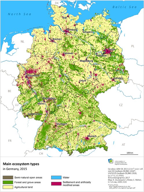
For the visual representation of the distribution of ETs at federal level, it makes sense to use grid cells of 1 km x 1 km. At smaller pixel sizes, an excessive number of differently categorised raster cells directly adjacent to one another can prevent the viewer from recognising large contiguous areas. Under the principle of dominant value, the raster cells of 1 km x 1 km are categorised according to the CORINE-Land-Cover (CLC) class with the largest proportionate area within the cell. This is not necessarily the largest undivided area occurring within the 1 km² cell. In this way, areas, such as meadows and pastures (CLC 231, sub-ET 32) in the Bergisches Land and in the foothills of the Alps, which are present in large numbers in the LBM-DE (Digital Land Cover Model for Germany), but which in each case often have only a relatively small individual size, can nonetheless determine the categorisation of this sub-ET, since the proportion of such areas is high overall. Similarly, high ratios of grassland for the above-mentioned regions are also found in the Thünen Atlas (Thünen Institute 2014).

The visual representation by the 1 x 1 km² raster grid only displays the rough spatial distribution of ET, but it did not serve as a calculation basis for the ET areas. The concrete areal ratios were derived from the vector-based spatial elements of the LBM-DE along with the additional small-scale and infrastructure elements from the ATKIS-Basis-DLM (Digital Basic Landscape Model from the Official Topographic-Cartographic Information System) (Suppl. material 3: The area and share of main ecosystem types and sub ecosystem types (ETs, see Tab. 1) in the German land cover model (LBM-DE) for the time periods 2012, 2015 and 2018. Linear elements such as small scale structures and infrastructures from the topographic-cartographic Information system (ATKIS) were added to the land cover model). One striking fact is that semi-natural open land has a share of less than 2%; accordingly, the areas and ratios of the CLC classes are marginal.

The introduction of linear infrastructures and small structures (Table 2) altered the areal sizes of some CLC classes compared to those given by LBM-DE. The area of the “roadway and rail networks” (CLC class 122) saw the largest increase, namely an additional 1,396,592.61 ha, due to newly-added surfaced and unsurfaced roads. Additionally the area of “watercourses” (CLC class 511) increased by 130,757.41 ha as a result of the additional watercourses. At the same time, other CLC classes decreased in size, especially the “non-irrigated arable land” (CLC class 211), falling by 363,700.13 ha. This was due, amongst other things, to the removal of farm roads from the calculation.

When considering the areal ratios for the year 2018, it becomes clear that the ratios of the main ETs correspond relatively well with known figures from Destatis land use statistics (Destatis 2019, Destatis 2020). Any disparities are largely due to differences in the definition of land use categories between the Destatis statistics and the applied geodata (Krüger et al. 2017). For example, comparing the extent of roads (CLC 122) in LBM-DE with that of Destatis, we note a disparity of approx. 300,000 ha, i.e. an area of 1.80 million ha for Destatis (Destatis 2019, Destatis 2020) compared to 1.54 million ha for the LBM-DE (with added roads, unsurfaced roads and railway lines). This difference could be due, amongst other things, to the fact that the two sources assume different standard widths and take different account of marginal areas, such as railway embankments and roadway verges.

In addition to the reference year 2018, the CLC classes for the years 2015 and 2012 were calculated using the indicated data (LBM-DE/ATKIS) and aggregated to sub-ET or main-ET. However, the relative brevity of the considered timeframe (three time periods) does not allow us to reliably determine any trends or shiftings, as these may be masked by methodological changes in the classification of land use and land cover in the LBM-DE (especially between the reference years 2012 and 2015) (BKG 2019b). Any interpretation of the ETs is also complicated by the fact that, for areas such as grassland, the classification of semi-natural open land changes from one time period to the next, even though no actual change of use has probably taken place (see above). In addition, the ATKIS data serving as a base data for the LBM have been changed by a process of systematisation lasting several years (a task completed in 2014), undermining the temporal comparability (AdV 2019). Thus we find a better agreement of the ET area sizes when comparing the years 2015 and 2018 than when comparing 2012 and 2015.

Main ecosystem types were assessed uniformly at federal level. In cases where it is appropriate and the data situation permits, the spatial framework was extended to the district level. The map representations were limited to the illustrations necessary for understanding.

A clear delineating of ecosystem types in a reliable manner is important for many current and emerging issues regarding ecosystem assessments and accounting, which ultimately helps to support decision-making. A number of good proposals have been made internationally in this context (Sect. 2), but it is still a dynamic field (Keith et al. 2020).

As discussed and confirmed in the SEEA revision process (UN 2020), the delineation of ecosystem assets should focus on classifying ecosystems from an ecological perspective. The consequence is that land cover alone is not sufficient. However, then the question arises - what kind of characteristics should be considered next in addition to land use? Should it be soils or better, water level or even relief? Soils would be good characteristics if we are looking at the ES for agricultural production; water level is relevant for carbon sequestration in peatlands; relief is of importance for erosion control and for scenic beauty. If we would use all these relevant characteristics for delineation, for each in part it would become important in the further process towards service accounting, then the result would subsequently be an enormous number of very small-scaled homogeneous spatial units.

However, it can be argued tha,t on the one hand, it remains uncertain if the results would have high accuracy, due to different data being collected at very different scales. Often, even they are not available at all or only in very coarse scales for the whole of Germany. On the other hand, all these resulting small homogenous patches would be aggregated again – but in what way – to make any meaningful statements about them with regard to their extent?

To conduct a nationwide analysis of ETs, in our opinion, it is more plausible to reduce the complexity and use ecosystem classifications, like that of the CLC ecosystem types. In general, land cover, in principle, quite accurately reflects the relevant characteristics of the ecosystems (e.g. forests on steep slopes, peat bogs in wet habitats, arable land on fertile soils etc.). If we need to refine the analysis in order to determine ecosystem conditions or services, however, it is reasonable to add additional information: has the land at the urban fringe converted to buildings resulted in higher natural soil productivity than average cropland? Is the water level of a mire ten centimetres higher or lower, which is decisive for carbon oxidation and greenhouse gas emissions? Is the cropland located on steep slopes so that soil erosion should be reduced by additional hedges or conversion to grassland?

If ecosystem services and ecosystem conditions are in question, additional information is obviously required. However, unlike in the ecosystem extent account, this information can then be used in a very targeted manner, depending on the respective land use, the status parameter under investigation and the ecosystem service that is assessed.

We have shown that the application to the German context, with practical realities considered, has transpired into emerging results. Although we start from the CLC classes, we use the German LBM-DE model, including some more characteristics than just land cover. Additionally, in the geodata system developed here, linear ATKIS elements (e.g. roads, watercourses or even small structures, such as rows of trees and hedges) are converted into polygons by means of buffering and integrating into the polygonal mapped ET and CLC classes. Care has been taken to ensure that no overlapping occurs, thus avoiding potential cases of double recording, thereby confounding the validity of result accuracy (Sect. 3.2).

However, a balance must be achieved between results that are sufficiently ecologically meaningful rather than being simply pragmatic and on which ET classification level this is relevant. We therefore believe that our proposed national system be processed in four levels (Main-ET, Sub-ET, CLC-classes, further subdivision into habitats to integrate biodiversity relevant information, Sect. 3). This would offer a flexible, but also simultaneously best appropriate, approach in this respect.

First evaluations have been realised and discussed (Sect. 4). In addition to the reference year 2018, the CLC classes for the years 2015 and 2012 were also calculated on the basis of the available data (LBM-DE/ATKIS), aggregated to Sub-ET and Main-ET, respectively, giving some results that allow for tentative interpretations. However, the brevity of the timeframe (three reference years) does not yet permit a reliable identification of trends or shiftings. Nevertheless, the results confirm the feasibility of conducting a national spatial monitoring of Germany’s ecosystems (Ecosystem Extent Account) in the future and of identifying possible changes on the basis of LBM-DE/ATKIS data.

The CLC classes defined in this way, when combined with other available information, are already sufficient for the evaluation of many ES (e.g. recreation, erosion control) and their conditions (e.g. hemeroby/natural condition,) . For example, in the case of natural soil fertility for the CLC class “arable land”, there is a combined analysis possible by overlapping the ETs with a number of other nationally-available datasets (including soil water balance, soil type, climate, slope inclination), which together enable an assessment of natural soil fertility, according to the Müncheberger Soil Quality Rating (SQR) (Mueller et al. 2007, BGR 2013a, BGR 2013b).

The system of ET/CLC classes (Table 1) is further underpinned by biotopes/FFH habitat types, for which extensive classification tables have been devised and developed (for an overview see Tab. B in Suppl. material 2). The recording and assessment of the condition (here especially biodiversity) of ecosystems can be further supplemented by the spatially explicit and representative data collected for each respective period.

To provide a spatial structuring of ecosystems, ‘condition indicators of landscape ecosystems’ can be used to measure the ratio of structural elements in the open landscape. This includes, for example, the IOER Monitor indicator “woodland-dominated ecotone density”, which reports on the density of linear elements, such as hedges, tree rows, woody plants and forest margins. It is precisely such elements that are of great ecological importance, as they represent transitional areas between ecosystems and are home to special communities of species that are thus particularly significant for the provision of ecosystem services.

Conversely, main roads or railway lines often have negative effects on the condition of ecosystems, as they act as barriers for wildlife and humans, thus impeding or even completely preventing key ecosystem functions. This aspect of the condition of ecosystems can be measured, for example, using indicators on landscape fragmentation as a whole or specifically forest fragmentation (see indicators on landscape fragmentation in the IOER Monitor: https://monitor.ioer.de).

Besides the classification system for ecosystem types (ETs), the table of the area of various ETs (Suppl. material 3, Table C) is the main result of our work. These datasets can form the basis for the regular reporting on the extent, condition and services provided by Germany’s ecosystems at national level. The approach for such an ecosystem accounting is in line with SEEA-EEA requirements (UN 2020). The Federal Statistical Office (Destatis) intends to further develop and implement the national ecosystem accounting system in the future. The recently-published IUCN Global Ecosystem Typology (Keith et al. 2020) will likely be a SEEA Ecosystems “reference classification” and it would be useful to bring our mapping and classification approach in correspondence with this IUCN typology.

Furthermore, we propose that the presented system to record the areal change in ecosystems should be developed into an integral component of biodiversity monitoring in Germany (Geschke et al. 2019). Due to the partial use of representative data, however, it is not suitable as a planning basis for concrete measures. In such cases, local data – for example, from the habitat/biotope mapping of the individual states – should be used (Grunewald et al. 2020).

For the long-term observation of ETs, a consistent and stable data-gathering methodology for the production of the main German data base, the LBM-DE, should be implemented to help realise a representative system of ecosystem monitoring. Only in this case, area changes of land use/land cover types can be mapped in a reliable manner. The results so far, which have been fully calculated for the German state area (terrestrial, inland surface waters, marine) on the basis of available data for the years 2012, 2015 and 2018, are still relatively uncertain with regard to trend developments or shifts, as these may be masked by methodological changes in the classification of land use and land cover (especially between the time periods 2012 and 2015) (B). There are also challenges in the consistency of the results (How can we deal with significant deviations from existing accounts, for example, forest and agriculture?).

Further challenges to be overcome are related to the degree of thematic detail that can be entailed, especially considering whether, which and with what kind of detail, functional characteristics of ecosystems should be included in order to support the realisation of the respective objectives at the national level (e.g. biodiversity protection, identification of services, prioritisation of damaged ecosystems to be restored, analysis of changes in the extent of specific ecosystems in Germany).