How to design a transdisciplinary regional ecosystem service assessment: a case study from Romania, Eastern Europe

Bálint Czúcz; Ágnes Kalóczkai; Ildikó Arany; Katalin Kelemen; Judith Papp; Krisztina Havadtői; Krisztina Campbell; Márton Kelemen; Ágnes Vári

doi:10.3897/oneeco.3.e26363

One Ecosystem : Ecosystem Service Mapping

PDF

Ecosystem Service Mapping

How to design a transdisciplinary regional ecosystem service assessment: a case study from Romania, Eastern Europe

Bálint Czúcz^‡,§, Ágnes Kalóczkai^‡, Ildikó Arany^‡, Katalin Kelemen^|, Judith Papp^|, Krisztina Havadtői^|, Krisztina Campbell^¶, Márton A. Kelemen^|, Ágnes Vári^‡

‡ MTA Centre for Ecological Research, Klebelsberg K. u. 3, H-8237 Tihany, Hungary

§ European Topic Centre on Biological Diversity, Muséum national d’Histoire naturelle, 57 rue Cuvier, FR-75231 Paris, Paris Cedex 05, France

| Milvus Group Association, Crinului Str. 22, 540343 Targu Mures, Romania

¶ Executive Agency for Small and Medium-sized Enterprises, European Commission, Place Charles Rogier 16, 1210 Saint-Josse-ten-Noode Brussels, Belgium

Corresponding author: Bálint Czúcz (czucz.balint@okologia.mta.hu)

Academic editor: Davide Geneletti

Received: 02 May 2018 | Accepted: 28 Aug 2018 | Published: 31 Aug 2018

This is an open access article distributed under the terms of the Creative Commons Attribution License (CC BY 4.0), which permits unrestricted use, distribution, and reproduction in any medium, provided the original author and source are credited.

Citation: Czúcz B, Kalóczkai Á, Arany I, Kelemen K, Papp J, Havadtői K, Campbell K, Kelemen M, Vári Á (2018) How to design a transdisciplinary regional ecosystem service assessment: a case study from Romania, Eastern Europe. One Ecosystem 3: e26363. https://doi.org/10.3897/oneeco.3.e26363

Abstract

There is a broad diversity of concepts and methods used in ecosystem service (ES) mapping and assessment projects with many open questions related to the implementation of the concepts and the use of the methods at various scales. In this paper, we present a regional ES mapping and assessment (MAES) study performed between 2015 and 2017 over an area of ~900 km² in Central Romania. The Niraj-MAES project supported by EEA funds and the Romanian government aimed at identifying, assessing and mapping all major ES supplied by the Natura 2000 sites nested in the valleys of the Niraj and Târnava Mică rivers amongst the foothills of the Eastern Carpathians. Major ES in this culturally and ecologically rich semi-natural landscape were determined and prioritised in cooperation with local stakeholders. Indicators for the capacities of individual services were modelled with a multi-tiered methodology, relying on the involvement of regional thematic experts. ES with appropriate socio-economic data were also evaluated economically. The whole process was supervised by a stakeholder advisory board endowed with a remarkable decision-making position, giving feedback and recommendations to the scientists at the critical nodes of the process, thus ensuring salience and legitimacy. In addition to simply presenting the dry facts about the approaches (assessment targets, methods) and outcomes, we also identify several key decisions on the design of the whole assessment process related to (1) the role of conceptual frameworks, (2) stakeholder involvement, (3) the selection of ES to assess (priority setting), (4) the development of models and indicators and (5) the interpretation of outcomes, for which we give a detailed description of the decision process. We found that conceptual frameworks can have a pivotal role in structuring and facilitating communication amongst the participants of a MAES project and that a broad and structured involvement of stakeholders and (local) experts creates a sense of ownership and thus can facilitate local policy uptake. We argue that priority setting and the development of indicators should be an iterative process and we also give an example how such a process can be designed, enabling an efficient participation of a broad range of experts and the collaborative development of simple ES models and indicators. Finally, we discuss several general issues related to the interpretation of results of any kind of MAES and the follow-up of regional MAES projects.

Keywords

MAES, ecosystem assessment, conceptual framework, mapping, transdisciplinarity, ecosystem condition, participatory approach

Introduction

Ecosystem services (ES) improve people’s individual and social well-being in many ways (MA 2005) and are indispensable for the healthy functioning of society and economy and their building blocks: local communities. In spite of this, we are losing ES at an alarming rate (Cardinale et al. 2012). Short-sighted decisions damage ‘nature’s free goods’, as concluded by a Transylvanian decision-maker in as early as 1786 (Molnár et al. 2015) in Sfântu Gheorghe, Romania - very close to the region where the ecosystem assessment presented in this paper took place. Amid the enormous environmental challenges of the 21^st century, this conclusion is more relevant today than it has ever been.

One of the reasons for society not being able to solve today’s environmental crisis is the ‘traditional’ way how society handles natural resources and environmental issues (Loorbach 2007). Each ‘sector’ is managed separately, by dedicated governance institutions, none of which has either the capacities or the mandates to handle overarching effects (Lyall and Tait 2005). A potential solution to this problem builds on the concept of ES that can serve as a boundary object (Star and Griesemer 1989) connecting the different sectors. Ecosystem service assessments offer a common platform to break down the silos and harmonise the otherwise isolated sectoral policies (Díaz et al. 2015). It is no surprise that the ES concept has been integrated into the most recent environmental / natural resource policies worldwide and there are several key policies addressing ES assessments specifically at an international and EU level (e.g. CBD’s Aichi Targets and the EU Biodiversity Strategy). A quantitative integration of ES into economic accounts (like GDP) is a major policy goal (Guerry et al. 2015), which could greatly influence all aspects of political and economic decision-making. Furthermore, mainstreaming the ES concept into general public communication (and enabling people to ‘think in ES’) can increase coping and problem-solving capacities (resilience) at a societal level (Díaz et al. 2015).

In this paper, we present and discuss several key ‘design questions’ of regional ecosystem assessment studies using a complex regional ES assessment as a case study. We present the Niraj-MAES assessment performed between 2015 and 2017 over an area of ~900 km² in Central Romania focussing primarily on the design decisions determining the assessment structure and the methods used. We lay particular emphasis on a few selected key aspects (“topics”) of the assessment process:

(Topic 1): the various roles of the conceptual framework (ranging from structuring the process to facilitating the communication, as discussed by, for example, Potschin-Young et al. 2018);
(Topic 2): the involvement of stakeholders and the integration of different knowledge forms (including stakeholder perceptions, unformalised expert knowledge, scientific literature and conceptual frameworks, e.g. Díaz et al. 2018, Dick et al. 2018);
(Topic 3): the selection of assessment priorities (including the decision on ES to be assessed) and the underlying process criteria (e.g. Ramirez-Gomez et al. 2015, Oudenhoven et al. 2018);
(Topic 4): the methods (models and indicators) available for quantifying ES and the criteria for choosing amongst them (selection criteria, as well as process criteria, e.g. Harrison et al. 2018, Wainger and Mazzotta 2011); and
(Topic 5): the integration of the diverse outcomes (ES models, maps, monetary values) into a common framework and the potential issues related to the interpretation of the outcomes (e.g. Dick et al. 2018, Olander et al. 2017).

In all of these key topics, we had to make serious design decisions during our assessment process, for which we could not find any easily accessible guidance in literature. Thus we made our own research, evaluated the options and brought our own decisions, and we learned a lot during this process. We think that our lessons can help others in similar situations and thus are interesting for the broad MAES community. Accordingly, in the following chapters we will

present the workflow of the Niraj-MAES assessment step-by-step, from the description of the assessment site and targets to the methods and indicators used for mapping to the final results of the assessment; and
integrate considerations (descriptions of the decision context, approaches considered and our final decision with justification) related to the five key topics highlighted above into the presentation of this workflow.

We do not intend to go into methodological details in any of the assessment steps with complex theoretical backgrounds (e.g. economic valuation), but we intend keeping the focus of the presentation on the structural design of the assessment process. Similarly, the primary outputs of the assessment process (indicators maps, monetary results) are also presented very briefly, only to the degree that is necessary to illustrate the methodological choices. The paper is concluded by ample discussion on the five key topics highlighted above.

Materials and Methods

Study area

The study area consists of four partly overlapping Natura 2000 areas (ROSCI0384, ROSCI0297, ROSCI0186 and ROSPA0028) comprising ~91,000 ha at the foot of the Eastern Carpathians between 301 m and 1080 m a.s.l. in South-East Transylvania, Romania. There are altogether ~203,000 inhabitants (average population density 68/km²) with 13% of the population concentrated in the six cities of the region. Settlements are mostly located along the two main rivers, the Niraj and the Târnava Mică. While agriculture is still a dominant source of income, official data show that few people earn their living from this economic sector. The relatively high share of natural and semi-natural habitats gives the landscape a ‘wild’ character, a consequence of the traditional land management practices that have been in use until very recently and can still be found in some parts of the study area. However, despite the deep affection the locals might have for the landscape, migration to urban areas is increasing, as better job and education opportunities are available there.

The vegetation has a transitional character between the lowland and the mountain regions of the Eastern Carpathians. The area is dominated by forests and pastures that were grazed traditionally by cattle, but nowadays rather by sheep. There has been an increasing tendency for land abandonment resulting in transient shrublands (encroached grasslands) in the place of former pastures, hay meadows or arable fields. Some of the hay meadows are still used for winter fodder production in cattle and sheep husbandry. Agricultural fields typically consist of a high number of small parcels reflecting historical land use and property systems, but larger plots cultivated by intensive modern agricultural techniques can also be found in the broad river valleys. Of the two main rivers, Târnava Mică is more natural, with broad meanders and gallery forests. The natural bed of the Niraj has mostly been destroyed in a series of recent riverbed corrections. Due to the lost meanders, the slope of the Niraj river has increased significantly, leading to strong erosion of the banks and a series of follow-up correction works.

Assessment principles

Conceptual framework (Topic 1)

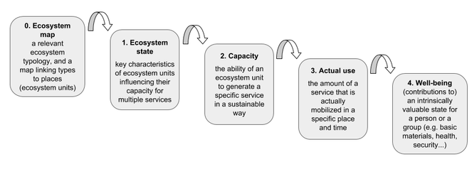
Throughout the assessment, we adhered to a conceptual framework (CF, Fig. 1) that can be seen as a customised and further operationalised version of the CF underlying the recommendations of the EU MAES working group (Maes et al. 2013, Maes et al. 2014) and the integrated ecosystem assessment (IEA) framework (Burkhard et al. 2018, Brown et al. 2018, Fig. 2) developed in the framework of the ESMERALDA project (Burkhard 2018) . We considered the most important roles of our CF that

Figure 1.

The conceptual framework (CF) of the Niraj-MAES assessment (based on Czúcz and Arany 2016), indicating consecutive steps of the assessment process.

Figure 2.

Matching the MAES assessment framework (a; Maes et al. 2014) and the ESMERALDA integrated ecosystem assessment framework (b; Burkhard et al. 2018) to our cascade-based conceptual framework (c; Fig. 1) and to our workflow (d; Fig. 3).

it creates a clear structure for the process of our work and the communication of our results,
it ensures compatibility with other similar assessments performed elsewhere and
it ensures conformity with the EU recommendations and thus complies with Romania’s national obligations towards the 2020 Biodiversity Strategy.

Following the ES cascade model (Potschin and Haines-Young 2011; La Notte et al. 2015; Czúcz and Arany 2016) underlying the MAES and ESMERALDA recommendations, our CF (Maes et al. 2014; Burkhard et al. 2018; Fig. 1) represents the various stages of the flow of the services from nature towards society. The starting point is rather technical: we need to have a spatially explicit account of what kind of ecosystems there are in the study area, which is represented by an ecosystem type map (level 0), classifying each land unit into the categories of an ecosystem typology perceived as meaningful by the locals. These ecosystems can be characterised with respect to a number of ecosystem condition aspects (level 1) that fundamentally determine their internal processes and operation. Appropriate condition enables ecosystems to provide services (capacity, level 2). However, the capacity of ecosystems to provide certain services is not the same as the services actually used (actual use, level 3) as the latter can be influenced by societal needs, ‘demand’ at a given place and time, as well as the human inputs expended to obtain services. The benefits of the services used then appear in the form of maintained or increased well-being in society (level 4, see all definitions in Suppl. material 1).

The key steps of this pathway define ‘entry points’ for interpreting and ‘measuring’ the flow of services from nature towards society. To implement this framework, we substantiated what kind of information we intended to assess at each level of this modified cascade framework (Table 1).

Table 1.

Download as

CSV

XLSX

Assessment goals as defined by the conceptual framework (CF): the type of information (number and type of indicators and the underlying typologies) sought by Niraj-MAES for each element of the CF.

Cascade level	Thematic dimension	Desired number of indicators	Spatial resolution
0. ecosystem map	ecosystem types	1 (a single map)	full (100 x 100 m)
1. ecosystem condition	condition aspects	1(-2) per condition aspect	full (100 x 100 m)
2. capacity	ecosystem services	1(-2) per ES	full (or aggregated)
3. actual use	ecosystem services	(1-)2 per ES (1 monetary and 1(-2) biophysical)	aggregated (or full)
4. benefits	ES, well-being dimensions	few (1 per ES and well-being dimension)	aggregated

To further implement the CF, we also created working definitions for several key concepts based on literature definitions and conscious harmonisation (Suppl. material 1). In line with these definitions, we also set down our attitude towards several 'hot questions' of ecosystem assessment practice discussed in the CICES manual (Haines-Young and Potschin 2018). For example, abiotic services (i.e. goods and services provided directly by the non-living physical environment without the assistance of biota, like mineral salts or extracted drinking water) were not considered as ecosystem services. We also excluded products derived from strongly transformed and principally human-controlled ‘industrial ecosystems’ (e.g. crops from intensive agriculture) which we considered to be on the ‘human side’ of the production boundary (Haines-Young and Potschin 2018), for several reasons:

as the process generating such goods is fundamentally governed by human management (through the above-mentioned inputs), the conceptual framework applied in this study (Fig. 1) would be very poorly applicable for the description and analysis of such services;
such goods require vast amounts of material and energy inputs from man (e.g. fertilisers, pesticides, agricultural machinery, fuel) which might easily exceed the contributions of natural systems to the production process (see, for example, the calculations in Bengtsson 2015);
contributions from natural ecosystems to agricultural production (e.g. pollination, pest control, soil fertility) are often considered to be (regulating) ES in their own right and taking into account both the regulating ES and the final crops as ES would qualify as double-counting (Boyd and Banzhaf 2007); and
agricultural goods constitute economic products that are already well represented in the currently existing economic accounts, so there is relatively little added value in (re)calculating / relabelling these already known values.

Accordingly, we considered such agricultural goods as internal products of the economy to which natural ecosystems contribute only indirectly, through other services (e.g. ensuring pollination, natural plant protection, maintaining soil fertility). Being potentially the most relevant, ‘soil fertility’ was chosen to be included in our assessment (compare also Albert et al. 2016; Rabe et al. 2016).

Participatory approach (Topic 2)

The use of scientific information for policy and resource management purposes should not be considered as a one-way knowledge transfer. A better model for the relationship of science and society in this process is that of a ‘joint knowledge production’ (Turnhout et al. 2007). From a policy perspective, the success of a research project resides in the use of its results by policy actors, influence on policy processes and impact on policy outcomes (Bauler 2012). It is actually the perception by key local, regional and national stakeholders (or policy actors) that determines the uptake of research results. There are three key components determining success in this respect: credibility (=scientific and technical suitability), salience (=ability to address user concerns) and legitimacy (=the political acceptability or perceived fairness of the process; Cash et al. 2003). In order to become influential, the research process needs to be perceived simultaneously and consensually as being legitimate, credible and salient by major groups of stakeholders (Bauler 2012). These criteria depend not only on the objective characteristics of the methods applied, but also on the perceptions of the relevant stakeholders. Accordingly, the research process should be considered as important as the results themselves, which is a common characteristic of post-normal science (Funtowicz and Ravetz 1993). Perceptions of credibility, salience and, particularly, legitimacy can be ensured by thorough stakeholder involvement throughout the research process. Intensive stakeholder involvement can also be considered as an example of extended peer review as proposed by Funtowicz and Ravetz (1997).

In this project, we aimed at involving a broad variety of stakeholders throughout the entire research process. The two main roles of the stakeholders (sensu lato) were:

to help to define priorities (what is perceived as relevant and what is negligible from the perspective of the local population) and thus ensure politically and socially relevant results; and
to assist in gaining a good system understanding (knowledge elicitation, how the different components of local society are interlinked with nature and economy).

In the second case (knowledge elicitation), the participating stakeholders were mostly selected according to their knowledge and expertise (local experts), while for the first case (prioritisation) opinions of the whole local population were regarded as relevant. We thus distinguished two ‘target groups’ for involvement: local experts with a thematic mandate related to their ‘expertise’ (that does not need to be based on formal training, in this context even an illiterate shepherd with a lot of traditional ecological knowledge can be considered as a local expert in grazing) and stakeholders (sensu stricto) that involves all locals, visitors and everyone else who has a stake in the well-functioning of the regional socio-ecological system. The involvement of local experts enabled us to capture complex nature-society relationships in the form of simple, but (locally) relevant models.

As a key element of making the Niraj-MAES research approach participatory, we relied on the help of an 'Advisory Board', comprising locals representing the most important economic and social sectors of the area (Box 1 in Suppl. material 2). The Advisory Board ‘supervised’ the entire assessment process, thus ensuring salience and legitimacy: every important step and result of the study was discussed with them and their suggestions were incorporated into the analyses, models and evaluations. The mapping and assessment process included, however, several further ‘participatory steps’ which had a vital influence on the outcome and success of the Niraj-MAES project, including an initial stakeholder analysis (Box 2 in Suppl. material 2), two ES prioritisation campaigns (Box 3 in Suppl. material 2) and a scenario planning exercise (Box 4 in Suppl. material 2).

To make the stakeholder involvement process equally as important as the results, leaders of the research had to be open-minded and reflect the needs of the stakeholders. The cooperation with the stakeholders started at the beginning of the research and was implemented by a locally embedded non-governmental organisation.

Assessment workflow

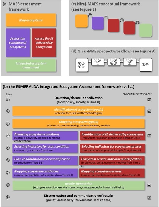
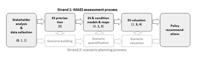
The structure of the research project that we designed, based on the guiding principles discussed above, is presented in Fig. 3. The scenario planning exercise, mentioned above, is not directly related to the implementation of ecosystem service mapping and assessment (MAES assessment) as put forward in the EU MAES working group recommendations (Maes et al. 2013, Maes et al. 2014). This is reflected by the fact that this exercise constitutes a relatively independent secondary strand of the project workflow, parallel to the MAES assessment. This paper primarily focuses on the process and results of the first strand, the MAES assessment process, while the stakeholder planning strand is described in detail in Kalóczkai et al. 2017 and Arany et al. 2016.

Figure 3.

The main workflow of the Niraj-MAES project, with major steps of the assessment process (Strand 1) linked to the boxes of the conceptual framework (numbers in parentheses, with bold numbers indicating primary focus (see Fig. 1).

The MAES assessment process predominantly follows the logic of the conceptual framework (Fig. 1) and the recommendations of the EU MAES working group, thus providing relevant results for high-level (regional, national and EU) policies. The complementary scenario planning process, on the other hand, primarily addresses the local level, involving broad groups of the local community. Accordingly, we considered the scenario planning strand as an equally important key element of the Niraj-MAES process, which can create an interest in the ES concept and the assessment process (Palomo et al. 2011) and enhance the exploration of future options for decision-making (Albert et al. 2017). The two strands are, however, interlinked at a few key nodes to maximise synergies (Fig. 3).

Setting assessment focus (Topic 3)

The selection of ES and the methods and indicators to measure them was done in an iterative process, gradually reducing the thematic scope of the assessment to a feasible set of well-defined ecosystem service indicators. This focus-setting process consisted of two main steps:

I: selecting / specifying the main 'topics' for the ES assessment (=the ES to be assessed);
II: implementing these topics by linking them to more specific indicators (=data and methods).

Selecting the services to be assessed

In order to make the ES assessment as locally relevant as possible, we started out with methods capturing the ES perception and priorities of a very broad range of local stakeholders (Kelemen et al. 2017), in an ES prioritisation process consisting of 3 main steps:

from the initial interviews of the stakeholder analysis (Box 2 in Suppl. material 2), we extracted a list of 'ES-candidates' (topics mentioned that can potentially be considered as ES);
these ES-candidates were then discussed and scored by the Advisory Board (Box 1 in Suppl. material 2) and an 'ES-shortlist' was selected; and
the shortlisted ES were finally ranked in a general preference assessment exercise (Box 3 in Suppl. material 2).

Based on individual rankings, we drew up an aggregated ranking of the services, describing the relative ‘value’ that the local population assigns to the different ES. The ranked ES shortlist, established through this process, was then revised, based on conceptual and technical considerations and discussed with the Advisory Board.

Selecting methods and indicators

For each ES valued by the locals as important to be included in the assessment, a matching indicator is needed that actually represents the service as closely as possible. For some services, this is a rather trivial choice, while, for others, some abstractions, combinations or specifications of certain aspects have to be made. To select indicators for ES mapping, we started out from both the results from the preference assessment process and the few ‘predefined’ ES that were named in our grant proposal (agricultural crop production, hay production, provisioning services from semi-natural ecosystems, carbon sequestration, habitat for biodiversity, recreational potential). Based on a number of methodological and conceptual considerations, several shortlisted ES were merged and some were considered to be most feasibly represented with condition indicators (Suppl. material 3). The indicators (as well as the underlying services / condition aspects) were then defined more precisely and appropriate methods were also identified for modelling them (Table 2). The selection criteria underlying our two-step decision process are summarised in Table 3.

Table 2.

Download as

CSV

XLSX

The list of ES indicators and ecosystem condition indicators selected for mapping in the Niraj-MAES project. Modelling approaches show the directions planned for model development at the stage of the ES selection, final models & indicators are specified in Table 6. CICES classes notifications follow Haines-Young and Potschin (2018).

short name	long name	definition of the ES indicator	cascade level	modelling approaches	CICES 5.1 classes
naturalness	habitat naturalness	The "naturalness" (incl. biodiversity and resilience) of the habitat. This ecosystem state influences the provision of several ecosystem services within and beyond the ones studied in this project, e.g. pest control, disease control, pollination.	1	statistical model (a Tier 2 index based on the modelled occurrence probabilities of some taxonomical groups of conservational significance)	-
landiv	landscape diversity	The habitat diversity of the broader landscape, which contributes to the persistence of several plant and animal species, as well to an aesthetically appealing environment.	1	statistical model (a Tier 2 landscape index: the diversity of broad habitat types under a moving window)	-
fertility	soil fertility	Fertility of the soil is a semi-persistent ecosystem state affecting the supply of several ES. In case of agro-ecosystems, it determines the ecosystem's potential contribution to the agricultural yield.	1	expert scores based on primary data (Soil Map of Romania (Harta Solurilor 1978))	-
hay	natural forage and fodder	Potential forage supply provided by the ecosystems through mowing or grazing. Cultivated or marketed roughage and grain feed are not included while grazing on fallow land and stubble as well as plants spontaneously occurring on waysides and banks are included in this service.	2	(1) matrix model (a Tier 1 statistical model based on expert scores and a habitat map)(2) enhanced matrix model (a Tier 2 statistical model with additional expert rules	1.1.3.1, 1.1.3.2
timber	wood and timber	Long-term timber and firewood provisioning potential of the habitat, assessed as a yearly average considering the whole lifecycle of the habitat, not taking effects of climate change into account.	2	(1) matrix model (a Tier 1 statistical model based on expert scores and a habitat map) (2) enhanced matrix model (a Tier 2 statistical model based on forestry production tables (Tabele de producție (Giurgiu et al. 2004))	1.1.5.2, 1.1.5.3
berry	medicinal and edible plants and mushrooms	Gathered mushrooms, fruits, berries and medicinal herbs provided spontaneously by the habitat. Cultivated plants and mushrooms are not included.	2	(1) matrix model (a Tier 1 statistical model based on expert scores and a habitat map) (2) enhanced matrix model (a Tier 2 statistical model based on structured exploration of plant habitat preferences)	1.1.5.1
honey	honey provision and pollination	Potential of the habitat to supply nectar and pollen for honeybees and so contribute to honey production.	2	(1) matrix model (a Tier 1 statistical model based on expert scores and a habitat map) (2) enhanced model (a Tier 2 statistical model based on habitat types and slope categories)	1.1.3.1
erosion	water retention & erosion control	Contribution of the land cover to slowing down the passage of surface water and thus to the recharge of regional groundwater resources and the mitigation of soil erosion.	2	(1) matrix model (a Tier 1 statistical model based on expert scores and a habitat map) (2) enhanced model (a Tier 2 statistical model based on habitat types and slope categories)	2.2.1.1
carbon	carbon sequestration	Sequestration and storage of atmospheric carbon by the habitat, as contribution to global climate change mitigation.	2-3	IPCC model (adapting a Tier 1 IPCC national greenhouse gas inventory model to the Niraj-MAES area)	2.2.6.1
tourism	tourism and local identity	Contribution of the habitat to the touristic attraction value of the area. Habitats allow recreation and create emotional bond in local people.	2	(1) matrix model (a Tier 1 statistical model based on expert scores and a habitat map) (2) enhanced model (an ESTIMAP-style Tier 2 statistical model based on the matrix model & additional rules)	3.1.1.1, 3.1.1.2, 3.1.2.4, 6.1.1.1

Table 3.

Download as

CSV

XLSX

Two sets of criteria for identifying indicators for the ES assessments. Phase I: criteria for selecting the 'topics' for which we need indicators; Phase II: criteria for selecting specific indicators (=data and methods) for each topic. CSL means credibility, salience and legitimacy; see Cash et al. (2003).

criteria	phase	CSL addressed	examples from Niraj-MAES
should meet stakeholder preferences / interests	I	legitimacy, salience	stakeholder analysis, preference assessment, SAB supervision
should meet policy interests	I	salience, legitimacy	sponsor expectations from grant call and promises in our grant proposal; SAB expressing local sectoral expectations/interests
should match conceptual considerations	I	salience, credibility	match to CF elements, exclusion of certain topics “based on MAES and CICES recommendations”
should measure what it states to measure	II	credibility, salience	meticulous ES and indicator definitions with an eye to data and methods, emphasised throughout all consultative steps and refined iteratively
should be supported by relevant expert opinion / knowledge	II	credibilty, legitimacy	expert workshops / consultations, SAB meetings; the involvement of local experts also considered to “assist in gaining a system understanding”
understandability, ease of communication	II	salience	transparent modelling techniques were favoured wherever possible, structured and thorough communication of all elements (indicator definitions, map explanations etc.)
data and methods availability	I, II	practical consideration	a very pragmatic criterion strictly applied throughout the ES identification and methods selection process
time and resource constraints	II	practical consideration	this made us exclude several options, e.g. Tier 3 models

Mapping and valuation

In the previous section, we have shown how we determined the questions and approaches in the focus of our assessment. In this section, we give a concise account of the specific data and methods we used, following the structure and logic set out in the Niraj-MAES conceptual framework (Fig. 1, Table 1).

Ecosystem map

The key input data layer consistent with the initial node of the Niraj-MAES conceptual framework is an ecosystem type map, classifying the study area into fundamental functional units (ecosystem / habitat types: level 0 in Fig. 1, see also Maes et al. 2014, and Suppl. material 1 for more precise definitions used). As there was no good quality ecosystem / habitat map readily available for our study area, we created our own map from scratch, based on the following data sources:

Google Satellite and Google Streets and Terrain layers (from the ‘open layers’ plugin of QGIS);
a land use map (own data from a previous project);
forest maps and data (official forestry administration data – but just for a few sites with Natura 2000 forest types).

To generate the ecosystem map, we first drafted an initial set of ecosystem types based on previous ES assessment experiences and our own understanding of the region’s landscape. This initial ecosystem typology was then gradually further specified and refined based on input from our expert groups, as we progressed with the generation of the ecosystem map. The most important principles of this process were the following:

the typology should be fine enough to reflect local reality (all major functional units of the Niraj-Târnava Mică landscape should be distinguished); but
the individual types should be clear and well-defined, forming a coherent and easily understandable (logical) set together;
the whole process should be feasible (given the available data and human resources); and
the final typology should be compatible with the MAES ecosystem typology (Maes et al. 2013).

The final ecosystem map assigns the dominant ecosystem types to each basic spatial unit of the study area (‘pixels’ of 100 x 100 m). The map was generated with QGIS (Quantum Gis 2.10.1. Pisa; QGIS 2016) in the Dealul Piscului 1970/Stereo70 coordinate reference system (the national CRS for Romania) and further refined in ArcGIS version 10.2 (ESRI 2011).

Spatial modelling (Topic 4)

In order to create maps of the ecosystem condition (level 1 in Fig. 1) or services (level 2), spatial data are needed. Such data can be either

external data from public data sources (whenever spatial data with an appropriate thematic, spatial scope and resolution are available for the project); or
modelled data (in all other cases – relying on loosely related external data and appropriate methodologies).

Models link biophysical data spatially represented by input maps with variables (indicators) describing the ecosystems with respect to a specific aspect of their condition or their capacity to provide a certain ES. In our work, we used models of three major model types: matrix models (tier 1 models), rule-based models and statistical models (latter two: tier 2 models, Grêt-Regamey et al. 2015, Grêt-Regamey et al. 2018).

Due to their simplicity and flexibility, matrix models are a particularly popular ES assessment technique (Burkhard et al. 2010, Jacobs et al. 2015). The only spatial input to the model is an "ecosystem map" (which is a simple categorical map relying on a locally relevant ecological (habitat), land use (management) and/or land cover classification) of the study area. The model itself is no more than a simple look-up table (‘matrix’) which links the ecosystem types to indicator scores. Matrix models are ideal for participatory model building involving local experts, but there are also several other ways to populate the matrix with scores (e.g. Bagstad et al. 2013). While participation gives the benefit of involving locals and enhancing uptake of results, this very simple approach might not reflect the complex processes underlying ES and the generation of ES precisely enough.

Rule-based models are an extension to matrix models. By identifying additional relevant spatial input data and including them into map calculation operations, the rough maps resulting from a matrix model can be highly refined. Similarly to matrix models, the transparency and intuitive nature of this model type can facilitate expert involvement. If experts are used for setting the rules and verifying the model outputs, then the resulting models can also be called expert models (Wainger and Mazzotta 2011). Depending on the number (and relevancy) of the rules included, this model is able to give a much better representation of reality. However, it basically does not give any estimate or measure of uncertainty.

Statistical models establish a correlative (statistical) relationship between a phenomenon of interest (e.g. the supply of an ES) and some readily available and presumably related predictor variables. In the most common setting, the phenomenon of interest is measured only at a few locations, whereas the predictors are known for the whole study area. In such cases, the statistical relationship captured by the model can also be used to estimate the phenomenon of interest in the unsurveyed parts of the study area. This type of model has the advantage that it is widely recognised within the scientific community and that it can also estimate measures of uncertainty. However, no local knowledge is included here and only statistical relationships can be shown, without any reflectance to causality.

In addition to the ecosystem map, there were several further spatial input data layers that we used in order to implement rule-based and statistical models (Table 4). All input data, including the ecosystem map, were converted to the same raster grid of 100 x 100 m cell size using ArcGIS (ESRI 2011) and QGIS (QGIS 2016).

Table 4.

Download as

CSV

XLSX

Overview of spatial datasets used for implementing rule-based and statistical models

feature/layer	source	sublayers / features used	data processing (model inputs)
roads	https://market.trimbledata.com	categories “trunk”, “primary”, “secondary”, “tertiary”, all “links”, “residential“ and “living street” from the layer “highway_line.shp”	secondary raster layer calculated with Euclidean distances -> "distance from roads"
rivers	https://market.trimbledata.com	the layer “waterway_line.shp” was used	secondary raster layer calculated with Euclidean distances-> "distance from water"
elevation	https://earthexplorer.usgs.gov	SRTM 30 m dataset	resampled to 100 m grid-size -> elevation, steepness, northing, easting
soil	Harta Solurilor 1978 (soil map of Romania)	Soil Map of Romania	raster layers describing various soil characteristics (genetic types, pH, texture) were created
grazing intensity	community / municipality administrations	number of cattle and sheep	created a raster layer which contained average grazing livestock density for each pixel of pasture or wood pasture habitat
surface reflectance	https://search.earthdata.nasa.gov	shortwave and NIR surface reflectance values from Landsat 8 OLI & TIRS imagery	calculated average reflectance values and reflectance variance for the 4x4 Landsat pixels around the centre of each grid cell of the ecosystem map from Landsat_8 bands 3, 4 and 5

To find the best models for each ES, we applied an iterative, adaptive and participatory strategy (Fig. 4). As a starting point, tentative modelling strategies were assigned to each ES / condition aspect (Table 2) as soon as they were identified. In most cases, this involved the development of an expert-based matrix model followed by a subsequent upgrade to a rule-based model and some expert validation. For an efficient implementation of this strategy, we organised two ‘matrix workshops’ with the participation of selected local experts (see Box 5 in Suppl. material 2). The maps created with the matrix models were instantly shown to the participating local experts for prompt feedbacks and corrections using the QuickScan software (Verweij et al. 2016). We used the opportunity presented by the workshops to elicit expert knowledge on potential ‘score influencing factors’ which we could later use for upgrading the matrix model into a rule-based model. In some cases, this was complemented with subsequent individual expert consultations (e.g. honey, hay, wood).

Figure 4.

Schematic concept of rule-based models chaining a matrix model (Burkhard et al. 2010) and subsequent adjustment rules.

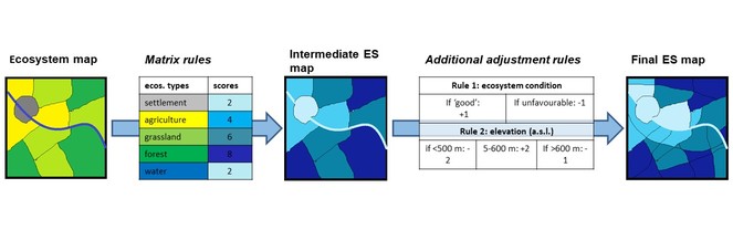
After a feasibility check and an update of the spatial data layers, we turned the influencing factors into rules and presented the structure and outputs (maps) of the resulting rule-based models to the SAB for verification. Recommendations received from the SAB members were then built into the model rules. The details of the final models are shown in Table 5 in the Results section. All models were implemented in R with add-on packages sp (Pebesma and Bivand 2005), rgdal (Bivand et al. 2016) and raster (Hijmans 2016).

Table 5.

Download as

CSV

XLSX

Overview of the ecosystem condition (EC) and ES capacity models used. Cascade levels follow Fig. 1 and tiers follow Grêt-Regamey et al. 2015, Grêt-Regamey et al. 2018.

ES/EC indicator	Cascade level	model type	model complexity (tier)	input data	external expertise involved
naturalness	1	statistical	2	habitat map, elevation, northing, easting, soil type, distance from roads, distance from water, reflectance (Landsat)	dedicated expert workshop
landiv	1	statistical (landscape)	2	habitat map (transformed)	individual consultations
fertility	1	rule-based	2	elevation, steepness, soil type	individual consultations
hay	2	rule-based	2	habitat map, naturalness, elevation, steepness, soil pH	matrix workshop
timber	2	rule-based	2	habitat map, elevation, steepness	matrix workshop, individual consultations
berry	2	rule-based	2	habitat map, naturalness, soil pH, soil texture, grazing intensity	matrix workshop, individual consultations
honey	2	rule-based	2	habitat map, naturalness, landscape diversity, soil fertility, elevation, grazing intensity	matrix workshop, individual consultations
erosion	2	rule-based	2	habitat map, steepness, grazing intensity	matrix workshop, literature
carbon	2-3	matrix	1	habitat map	literature
tourism	2	rule-based	2	habitat map, naturalness, landscape diversity, elevation, distance from roads, distance from water	matrix workshop

Table 6.

Download as

CSV

XLSX

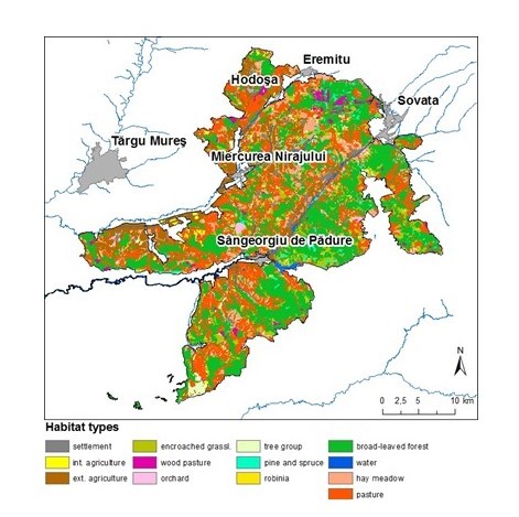
The final list of ecosystem (or habitat) types distinguished in our ecosystem map. MAES types follow Maes et al. (2013).

habitat category (ecosystem type)	definition	criteria for delineation	MAES type	relative area
settlement	villages, outer areas with gardens and single farms	easily recognisable (on the basis of the satellite images)	urban	1.7%
intensive agricultural	intensive, large arable fields (patches >10 ha)	homogenous arable land patches larger than 10 hectares (on the basis of the satellite images)	cropland	0.5%
extensive agricultural	mixed agricultural mosaic of small patches of various uses (patches <10 ha)	any patchy landscape, with patches smaller than 10 hectares (on the basis of the satellite images)	cropland	12.7%
pasture	pastures, grazed grasslands of different degrees of degradation	large patches of homogenous grassland areas (on the basis of the satellite images, at scales of 1:9000 and 1:11 000), sometimes with visible signs of overgrazing (eroded parts in the fields)	grassland	26.7%
hay meadow	hay meadows	separated from pastures based on the land use map	grassland	6.9%
encroached grassland	shrublands, abandoned grasslands encroached with shrubs	grassland patches with more than about 30% covered by shrubs (estimated visually on the satellite images at the scales of 1:5000 and 1:11 000)	grassland, woodland and forest, heathland and shrub	7.6%
wood pasture	solitary trees in grassland patches	easily recognisable by the solitary trees in grassland patches (on the basis of the satellite images)	grassland, woodland and forest	1.6%
orchard	abandoned or extensively used fruit tree plantations/vineyards	areas with tree or shrub plantations in rows, visible on the satellite images (at a scale of 1:11 000), which were also marked as fruit tree plantations or vineyards on the land use map	cropland	0.4%
tree row	group of trees/small forests/tree rows/galleries along small valleys	small groups of trees, thick and continuous shrublands, galleries along valleys and rivers located in larger grasslands, agricultural lands or along the riverbanks (on the basis of the satellite images)	woodland and forest	3.8%
pine and spruce forest	coniferous plantations	within forests: extreme dark colours on LANDSAT 8 false-colour maps (Bands 5, 4, 3); checked with forestry data where available	woodland and forest	1.3%
robinia forest	robinia plantations	within forests: light colours on LANDSAT 8 false-colour maps (Bands 5, 4, 3); checked with forestry data where available	woodland and forest	0.1%
broad-leaved forest	deciduous forests of native tree species	all large forest areas (on the basis of the satellite images), apart from coniferous forests and robinia plantations	woodland and forest	35.6%
wetland and water	major rivers, lakes and fisheries, including the reed banks	major rivers within the project area (Niraj and Târnava Mică) and the lakes and fisheries, including the reed banks (as these surfaces were relatively small) (on the basis of the satellite images and Google Terrain layer)	rivers and lakes, wetlands	1.1%

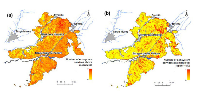
The resulting ecosystem service maps express the extent to which certain habitats are able to contribute to securing a specific service. By juxtaposing these maps (by spatial overlay of individual ES maps), the parts of the landscape become comparable and locations and regions that are particularly important for the provision of specific services can become visible (e.g. Eigenbrod et al. 2010, Nikolaidou et al. 2017, Rabe et al. 2016). To facilitate this kind of comparison, we also prepared two overview maps that show, for every single point (pixel) of the study area, the number of services being provided at above average (the upper 50%) or outstanding (the top 10%) performance, thus highlighting regional ‘hotspots’ for ES provision.

Aggregated valuation (Topic 5)

Following the spatial modelling steps in which we compiled maps of ecosystem condition and resulting capacities to deliver ES (cascade levels 1 and 2), we evaluated the actual use and the value dimensions of ES (cascade levels 3 and 4) in an aggregated (non-spatial) way. Here, single quantitative values for each ES were calculated, which characterise the ‘magnitude’ of the ES over the whole area from a specific perspective. To give an aggregate evaluation of the actual use, we relied on external indicators from public statistical data that quantitatively describe the actual harvest and/or consumption of the ES in the study area in terms of an appropriate numeric unit.

In order to give a complete account of the benefits generated by ES, all major aspects in which they are useful to society (e.g. health, security and material well-being) need to be considered (Olander et al. 2018). In our work, we considered several biophysical, social and economic aspects of well-being, thus implementing an integrated valuation approach. As this has already been mentioned, several steps of the research process constitute a form of ecosystem service valuation by themselves: the ES prioritisation exercises (Box 3 in Suppl. material 2), as well as the scenario planning process (Box 4 in Suppl. material 2) can be considered as extensive social valuation exercises yielding comparable ‘importance scores' for the studied services along a common ordinal scale. To make the assessment more comprehensive (and partly also to meet the donor expectations), we complemented these social value dimensions with economic values using simple valuation techniques.

The primary reason to ‘aggregate’ over the whole project area was that both publicly available statistical data and social valuation results were available at a coarse spatial resolution.

Considering money as a special indicator dimension, we tried to assign monetary values both to the capacity and the actual use levels (Fig. 1) of the studied ES. To monetise the capacities, we first had to convert the scores obtained from the matrix and/or rule-based models to biophysical units (ideally to the same units which were used to characterise the actual use of the ES), based on expert consultations and literature resources. (In this step, the knowledge of the local experts that ensured local validity was of particular importance.) The converted biophysical capacity metrics were then aggregated over the whole study area to make them comparable to the actual use units. We used various methods for the monetary valuation of capacities and actual use:

For most of the provisioning services (wood and timber, natural forage and fodder, wild plants and mushrooms and honey), we used market prices as the basis of our calculations. In this case, the concerned ecosystem service needs to have a market, where it can be sold. In the valuation process, we strived to consider least processed products and average prices measured on local markets in the past few years, i.e. prices realistically available to local farmers. We aggregated the monetary benefits of specific habitats for the entire area, thus arriving at a total amount that is provided to the local and national economy by the area as a whole.
We also used market prices for the valuation of carbon sequestration, based on international emission trading systems. In the case of the other regulating services which were directly or indirectly mapped through our ES indicators (water regulation and erosion control through our indicator for water retention and pollination partly mapped through our indicator for honey), we did not attempt to perform an economic valuation. The data needs and methodological challenges necessary for the valuation of these services were clearly beyond the reach of this project.
For the valuation of the only cultural ecosystem service assessed (touristic attraction) we used the travel cost method. This method is based on actual consumer behaviour (‘revealed preferences’) and valuates the services based on them. Travel costs address ‘products’ related to getting access to the cultural benefits of natural resources, as a substitute for market price. To value the recreational services of a given area, information is needed from a large and representative sample of visitors/tourists, for which we made a dedicated survey (Czúcz et al. 2017b). Based on the individual preferences, a demand curve can be drawn, which can reveal the consumer surplus reflecting the value of the underlying service.

Monetary valuation of ES is a very broad and deep topic and we do not want to argue about its general usefulness or go into any methodological details here. In this paper, we only present our monetary valuation process to the degree which allows us to discuss its role in our case study and other regional ecosystem assessments:

how do monetary values fit into the overall assessment context (what is their relationship to other indicators, to local expert knowledge, how to communicate them to stakeholders etc.); and
for which ES did we apply monetary valuation (and why) and which broad “families” of monetary valuation techniques we chose (and why).

All further details on the methods and data used for the monetary valuation can be found in Czúcz et al. 2017b.

Results

In the following paragraphs, we briefly show the most important direct outcomes (primary results) of the Niraj-MAES project. However, given the methodological focus of this case study description, the methodological lessons (Topics 1-5) are no less important for this paper. These methodological results will be described in the next section (Discussion), whereas this section focuses primarily on those aspects of the primary results, which are also necessary for the methodological discussions. A more detailed record of the primary results can be found in Arany et al. (2017) and Kelemen et al. (2017).

Priority setting

Based on the initial interviews of the stakeholder analysis (Box 2 in Suppl. material 2), we could identify 47 'ES-candidates', which were screened and condensed down to a shortlist of 12 regionally important ES by the SAB (Box 1 in Suppl. material 2): water regulation, tourism, local identity, wood and timber, wild edible plants, soil fertility, extensive orchards, pollination and honey, climate regulation, hay and fodder, erosion control and game/hunting. These shortlisted ES were ranked in two parallel ES prioritisation exercises (Box 3 in Suppl. material 2), which addressed the preferences of the local population in general and the local economic actors, respectively. Priority ranking of ES were similar in both groups with the importance of ‘water’ being perceived as outstanding (a popularity of 72% in both surveys). Water was followed by touristic attraction (49%) and local identity (48%) in the general population, while entrepreneurs regarded local identity to be more important (62%), followed by timber provision (52%), which slightly preceded tourism (48%). Besides, more than 40% of respondents considered wood and timber, wild plants and mushrooms, honey and pollination, as well as carbon sequestration important in the general population, while only pollination and carbon sequestration reached this threshold within entrepreneurs (see the detailed outcomes below in Table 7).

Table 7.

Download as

CSV

XLSX

Key results of the social and economic valuation of ecosystem services.

	Socio-cultural valuation				Biophysical and economic valuation				Expected future changes in the services⁴
	Importance perceived by the population¹ (%) and the most common justifications		Importance perceived by economic stakeholders² (%) and sectors most affected³		Economic value (million EUR/year)
					methodology	capacity⁵	actual use⁶	actual use / capacity ratio	trend	uncertainty
Wood and timber	45%	raw materials, livelihood, building materials, oxygen production, clean air	52%	logging, wood processing, plant production, livestock farming	capacity: based on average annual increase during the economic life cycle of forests, without discounting	4.4	3.3	75%	slight increase	small
					actual use: based on logging data
Natural forage and fodder	28%	livestock production, livelihood	28%	livestock farming, plant production	based on market off-take of grazing sheep and cattle populations	–	3.1		slight increase	small
Wild plants and mushrooms	44%	health, medicine, food, livelihood, recreation	32%	(there was none amongst sectors consulted)	average quantities calculated based on the number of collection permits issued, multiplied by average buying-in prices per species	–	1.4		strong decline	large
Honey and pollination
Honey and nectar	41%	pollination, health, food, healing properties, livelihood, experience	26%	livestock farming (beekeeping)	capacity: based on the estimated annual quantity of honey that can be collected on average in different habitats of the area	1	0.8	80%	constant	medium
					actual use: number and average production of registered bee colonies
Pollination			40%	livestock farming, plant production		–
Water retention
Water regulation	72%	basic needs, water quality, health, wildlife, food, livelihood (fishing), recreation	72%	all sectors		–			slight decline	large
Erosion control	25%	landslides, soil erosion control, basis for food production	38%	livestock farming		–
Carbon sequestration (climate protection)	40%	climate change as a global problem	46%	livestock farming, plant production	drawing on the methodology of the Romanian national greenhouse gas inventory, based on emission-trading market prices⁷	1.3	1.3		slight increase⁸	small⁸
Touristic attraction and local identity
Tourism	49%	livelihood, potential for development, acquiring knowledge, experience, beauty, clean environment, valuable natural environment	48%	food retail, catering, tourism, livestock farming, plant production	based on the number of visitors in the area and the amount of money spent by them for touristic or recreational purposes	–	3.6		constant	small
Local identity	48%	respect for traditions, emotional bond, national self-awareness	62%	food retail, catering, tourism, plant production		–			–	–
1: % of respondents who ranked the specific service amongst the 5 most important
2: mean dependence score assigned by business actors (% of the maximum score)
3: sectors that assigned a score of above 50%
4: the average trends of expected changes in the four possible scenarios (for a detailed description of the scenario planning process see Arany et al. 2016, and Kalóczkai et al. 2017)
5: estimated economic value of ecosystem service capacities per year
6: estimated economic value of current actual use in the year 2015
7: carbon sequestration, similarly to other regulating services, is "used" without conscious human involvement, which is why actual use can be considered equivalent to capacity
8: carbon sequestration, a service difficult to interpret at the local level, was not included in the scenario planning process, but the results obtained for the "wood and timber" service in terms of trends and uncertainty can be considered valid for this service, too

Ecosystem map

The final ecosystem types and their definitions are described in Table 6 and the ecosystem map is shown in Fig. 5. More than one-third of the region is covered bydeciduous forests and over 40% is some kind of grassland (pasture, meadow, encroached grasslands or wooded pasture). Only 13% of the studied four Natura 2000 areas is cultivated agricultural land. Just 3.5% of the agricultural land is under intensive cultivation, while the overwhelming majority (96.5%) is extensive small-scale agriculture. A great proportion of the studied 91,000 ha is covered with some kind of natural vegetation, which provides a solid basis for high biodiversity.

Figure 5.

The final ecosystem map consisting of 13 ecosystem / habitat type categories.

Condition and capacity

An overview of the final models for ecosystem condition and ES capacity is presented in Table 5, with particular focus on model type, the data used and the level of expert involvement. In order to reflect the dependence of ES capacity on proper ecosystem conditions, ecosystem condition indicators (e.g. naturalness or soil fertility) were included in the modelling rules wherever it was considered appropriate. In addition, feed-back with actual data on usage intensity was added (in order to connect condition with cascade level 3) where this was feasible/logical. For example, on grasslands, the provisioning capacity of hay or honey can be severely limited by degradation due to recent overgrazing, which is thus reflected in the ES capacity models. Vári et al. 2017 give a more detailed overview of the fitted models, the underlying assumptions and the techniques applied, as well as the resulting maps.

Fig. 6 provides an overview of the ES ‘hotspots’ of the Niraj-Târnava Mică region. Most of these areas are located on higher, varied terrains and consist in a mosaic of different natural and near-natural habitats. It seems that all habitats are inherently ‘multifunctional’, i.e. capable of providing several different services, with the only exception being the intensive agricultural areas, the main crops for which we did not consider ecosystem services.

Figure 6.

Overview of ecosystem services in the Niraj-Târnava Mică region: the number of services provided (a) at an above average (>50%) level or (b) at an outstanding (>90%) level for each basic spatial unit (pixel).

Actual use and benefits

In Table 7, we summarise the key aggregated results of the Niraj-MAES assessment process. In this table we present

the perceived importance of the services amongst the general population and local businesses;
a short summary of the data sources and methods identified as most appropriate for generating aggregated ES capacity and actual use indicators in natural (biophysical) units;
the estimated monetary values of these capacities and actual uses and the ratio of actual use to capacity wherever this was feasible; and
the expected future trends of each ES, as an outcome of the scenario planning strand of the project.

Czúcz et al. (2017b) describe all assumptions and techniques underlying the estimation of aggregated capacities, actual use and monetary values presented for each ES. The detailed process and results of the scenario planning strand are described by Arany et al. (2016) and Kalóczkai et al. (2017).

Discussion

In the previous chapters, we presented an operative and participatory process for a regional ecosystem assessment. In addition to concisely presenting the main steps, we gave a relatively detailed discussion and justification for all major design decisions already in the materials and methods section. Here we would like to discuss some further lessons we learned from the whole process regarding three major aspects: designing the assessment, practical methodological choices and caveats in interpreting the results.

Top-down vs. bottom-up (Topics 1-3)

Our key lesson regarding assessment design is that bottom-up and top-down elements throughout the assessment need to be in a delicate balance in order to meet the triple criteria of salience, credibility and legitimacy (Cash et al. 2003, Oudenhoven et al. 2018) in the end. Regional relevance (credibility and salience in a local context) and legitimacy are ensured through an influential stakeholder integration (Topics 2 & 3, bottom-up decisions), whereas salience in a high-level context (e.g. from the project funder’s perspective) is ensured by a close adherence to the CF: every element of the assessment process needs to be matched to an element of the CF in the clearest and most logical way possible (Topic 1). This sets a more substantial and more precisely defined role for the CF than the one proposed by Potschin-Young et al. (2018), who argue that the CF should be used as a tool for for structuring and prioritising work, ‘re-framing’ perspectives, an ‘analytical template’ and a common reference point for discussions. Ideally, by determining the overall structure and the types of information sought, an appropriate and broadly accepted CF could ensure compatibility for all ecosystem assessments worldwide. This could facilitate a broader picture emerging from many small assessments, which would make regional assessments more valuable for high-level (EU, global) policies. This would necessitate, however, a revision of the simple cascade model (Costanza et al. 2017) and more research on optimal CF structure(s) (Potschin-Young et al. 2018).

To ensure this adherence and establish the right balance between bottom-up and top-down is the responsibility of those scientists performing the actual assessment. Being a ‘model’ itself (see definition in Suppl. material 1), the ‘CF’ is necessarily a simplification of the complex world and it is not always obvious how real life objects and phenomena should be rendered in the simplified categories of the CF. Even determining whatan ES really is and what should rather be considered as a condition aspect or a benefit can be non-trivial and context dependent (Potschin-Young et al. 2017). Furthermore, many ‘ES-as-perceived-by-the-locals’ are related in delicate ways (served in bundles or generated by related processes, depend on the same ecosystem characteristics, are consumed together or are just different benefits/aspects of the same bundle), which can compromise further modelling and discussion efforts. All of these make it really challenging to start out from ‘locals-defined’ ES in an ES assessment (and that is why many studies simply start out from a predefined ES list – e.g. Rabe et al. 2016, Norton et al. 2012, Boerema et al. 2014). On the other hand, balancing top-down with bottom-up, i.e. integrating the local context is the only way of making the whole assessment really locally/regionally relevant (credible and legitimate; e.g. Kati and Jari 2016, Ramirez-Gomez et al. 2015). To balance these two approaches, high-level flexibility was required from the scientists and willingness of cooperation and openness from the locals. To bring together the interests of these two groups, there was a need for a locally embedded facilitator who supported the whole process by intensive activity and communication. Once clearly communicated and justified with CF considerations, however, top-down perspectives were understood and accepted by local stakeholders (e.g. merging two services under a single indicator or placing a ‘service’ into the condition box). Thereby, these discussions turned into a learning process, thus improving ‘ES-thinking’ amongst key actors of the region and promoting the development of a shared understanding related to relevant regional environmental issues and their potential solutions. The combination of bottom-up and top-down aspects in scope-setting and process design thus became mutually instrumental for both the researchers and the stakeholders participating.

Another major lesson learned from matching locally raised issues to CF boxes was related to the role and importance of the integration of ecosystem condition into the assessment. Being at the starting point of the cascade, condition, if defined and handled correctly, can indeed play a central role in making the assessment meaningful. If interactions between ecosystem condition and ES capacity are not included in the models, we lose the opportunity to show the effects of a changed condition on the potential of the ecosystem to provide ES. To be in a position to include conditions, we need a functional definition which reflects (and thus implements) the CF context: as ecosystem condition, we considered those ecosystem characteristics (state descriptors), which are not services themselves (i.e. have no clear ‘benefit aspects’), but rather influence the provision of multiple ES at the same time (see the exact definition(s) in Suppl. material 1. The importance of condition can also be formulated from a systems theory perspective: a system model connecting nature and society with two layers of internal nodes (condition, capacity) can provide a much better (more realistic) representation of system functioning than a model with a single ‘internal node’ layer (just ES capacities) would be able to do (Wainger and Mazzotta 2011, Olander et al. 2017). Accordingly, if condition dimensions are adequately identified, including appropriate indicators and integration into ES capacity models, then the whole assessment becomes more ‘realistic’ and meaningful for policy applications. Perhaps the most important aspect of this improved policy-relevance, is that sensible ecosystem condition indicators make it possible to quantify potential conservation/restoration targets and achievements, which is a central element of many key policy targets (e.g. to measure achievements, as in EU Biodiversity Strategy: Target 2 or Aichi Target 15; or to create flexibility through compensations, as in EU Biodiversity Strategy: Action 7 or SDG 15: Target 3). Furthermore, a meaningful interpretation of condition and the documentation of how it influences ES can also provide easily understandable key messages of the ecosystem assessment for the general public. It does matter in what state nature is around us – this determines the services we receive from nature and, ultimately, our own well-being.

Practical methodological choices (Topic 4)

A further major lesson that we can derive refers to the power of simple approaches, algorithms and proxies - in case of very limited data, when there is no possibility to apply more demanding complex methods, they are often of key importance. Simple but locally customised models can offer an optimal balance between ‘quality’ and ‘feasibility’ (Wainger and Mazzotta 2011, Olander et al. 2017) and they also allow for more interaction with local experts. The involvement of local thematic experts can create a sense of ownership and legitimacy to the process, thereby potentially also promoting a change of attitude (Dick et al. 2018). As the matrix approach is rather simplistic, the whole assessment procedure remains more transparent and easier to communicate (Dunford et al. 2018). In our assessment, any time when there was a choice between a more precise, more technical approach with less participation and a more participatory solution, we chose the latter.

A matrix workshop (as described in Box 5 in Suppl. material 2) can be an efficient way of ‘mass producing’ tier 1 matrix models involving key local expertise. In our experience, ordinal scale -matrix models are useful for valuation of the targeted ES in the first round, in order to approach dependencies and relationships. By converting the ordinal scales into biophysical units (where this was possible), the models became more concrete, less subjective and better manageable in terms of realistic assessment. We suggest that after the first round of matrix-scoring, the ordinal scale ‘values’ of the models should be converted as soon as possible into biophysical units (e.g. based on literature or expert judgements) for further validation, as well as the generation of adjustment rules that allow the matrix model to be developed into a tier 2 rule-based model. Adding more iterations (with possibly new local experts and/or stakeholders) refines the outcomes. Apart from being more concrete, models in real biophysical units also have the advantage that they can help to circumvent issues related to the non-additivity and non-linearity of ordinal scales, which are, unfortunately, commonplace in contemporary ES assessments and even suggested in high-profile publications (Burkhard et al. 2014). This is a prerequisite for performing valid and meaningful arithmetics (e.g. subtracting capacity from actual use (as in Hein et al. 2016) or setting up adjustment rules in a mathematically correct way). Ignoring this is not just incorrect, but it might easily lead to wrong conclusions regarding the sustainable use and capacities of ecosystems.

This approach – matrix models developed in expert workshops – relies mainly on the availability of a rather large number of locals showing expertise in some of the ES to be assessed. Successful involvement requires access to local social networks (which was provided by the local NGO in our case) and a lot of personal effort communicating the importance of their participation to local experts / stakeholders. In cases where data, biophysical models and modelling expertise are more accessible, local adaptation (including customisation, fine-tuning, verification, see e.g. Zulian et al. 2018) of a detailed biophysical model can also be an option, which is superior to simple (local) expert-based models. However, most of the tools in the widely used ES toolkits (e.g. InVEST – Posner et al. 2016, ESTIMAP – Zulian et al. 2013) are also tier 1 or tier 2 rule-based models, very similar in structure to the models used here. For example, the model we developed for calculating carbon, is very similar in structure to the InVEST Carbon Storage and Sequestration model, both of which rely on the same IPCC approach (Posner et al. 2016, Vári et al. 2017) and the Niraj-MAES model for estimating honey provisioning capacities is structurally very similar to the ‘floral abundance component of the ESTIMAP pollination module (Zulian et al. 2013, Vári et al. 2017). Co-developing models with local experts creates additional flexibility: it makes those locally relevant ES also accessible, for which there are no available modules in any major modelling toolkit (e.g. “natural forage and fodder” and “wild plants and mushrooms” in our case). Data and resources which would be needed for more detailed biophysical modelling were also an issue in our Eastern-European context and the additional benefits of a broad participatory process were also highly rewarding for the local NGO partner. Accordingly, whenever a choice has to be made between the greater biophysical realism of complex biophysical models and the potentially less precise but more inclusive and democratic ‘matrix + rules’ approach, we chose the latter (see also Dunford et al. 2018).

Caveats in presenting and interpreting the results (Topic 5)

The structure of MAES assessments partly reflects the complexities of socio-ecological systems. It is little wonder that the outputs of such complex processes are also of considerable complexity and thus need careful and knowledgeable interpretation. Especially for stakeholders or decision-makers with little previous experience with ecosystem assessments, there is a high risk of inadvertent misinterpretations. This again creates additional responsibility for the scientists coordinating the research: to take a proactive approach in annotating and discussing the outputs in a form that minimises risks for misinterpretation. This also involves creating summaries at various levels of detail for various audiences – including, for example, a general high level ‘summary for policy makers’, various sectoral ‘policy briefs’ and a detailed ‘project report’ thoroughly explaining all materials and methods and justifying all design decisions (a practice also followed by us in the Niraj-MAES project). The higher-level summaries also need to be carefully referenced back to the facts and discussions documented in the more detailed ones. These are, rightfully, standard practices of all major international institutions (e.g. IPCC, IPBES – Compagnon and Cramer 2016) which could also greatly facilitate policy uptake in local / regional assessment contexts. However, such protocols alone cannot guarantee that policy-makers will be able to correctly interpret all assessment outputs. There are several further potential ‘(mis)interpretation pitfalls’ related to the particularities (characteristics, diversity) of ecosystem services and their quantification. The way how these issues are handled can greatly influence the usefulness of the outputs. In the next couple of paragraphs, we will discuss such issues related to the synthesis / presentation of assessment results for which we have learnt relevant lessons during our work on Niraj-MAES.

Defining hotspots by spatial overlay of individual ES maps is a popular option for spatial synthesis in ES mapping and assessment projects (e.g. Eigenbrod et al. 2010, Nikolaidou et al. 2017, Rabe et al. 2016). However, this implies bringing all ES maps to a ‘common denominator’ first. This is only straightforward if all ES are monetised, which is a very rare situation – but in most other cases no good/default way exists for this. Our approach (cutting the maps at specific percentiles – see also e.g. Qiu and Turner 2013) can be a "quick and dirty" solution which comes at the price of considerable information loss. Nevertheless, such hotspot maps assume equivalence amongst all studied ES and flatten out their scales via binarisation, which renders the interpretation of such hotspot maps dubious. (e.g. are 5 services at 51% of their regional range better than a single ES at regional maximum (100%) and some others at 40%?) Hotspots should be supported by verification (‘ground-truthing’ – e.g. by local experts, ground data or remote sensing), especially if there is an intention to propose practical suggestions related to ES hotspot regions. A practice of 'hotspot verification' could even be integrated amongst the recommended practices in the final phases of ES assessment studies.

Interactions (synergies/trade-offs) between ES are other hot topics discussed in many ES studies. However, in many cases such trade-off analyses are based on a post-hoc examination of the spatial patterns of the overlaid ES maps (e.g. Becerra-Jurado et al. 2015, Albert et al. 2017, Lee and Lautenbach 2016 – called as 'spatially explicit ES bundle approach' by Raudsepp-Hearne et al. 2010), which is essentially an extension of the hotspot maps discussed above. Spatial patterns might, nevertheless, be caused in many different ways, including correlated (or identical) background factors (like soil, land use or altitude) or model input variables (like accessibility) which might lead to trivial, uninformative or even misleading correlation patterns (Tomscha and Gergel 2016, Marsboom et al. 2018). ES belonging to an ES bundle (MA 2005, Bennett et al. 2009), as, for example, freshwater fishing and recreation (Smith et al. 2017), carbon sequestration and timber provision (Smith et al. 2017, Vári et al. 2017) or pollination and honey production (Vári et al. 2017), can be seen as real interactions, but are still not as interesting for local governance and policy as the ‘real’ synergies or trade-offs, where harvesting one service compromises the capacity of the source ecosystem to supply some other ES (Spake et al. 2017, Turkelboom et al. 2018). To identify such ‘real’ trade-offs and synergies, something more is needed: e.g. stakeholder interviews to explore and confirm trade-off / synergy mechanisms (Martín-López et al. 2012, Lee and Lautenbach 2016, Turkelboom et al. 2018) or at least a detailed analysis of the spatial models and their input data to exclude other sources for spatial correlation patterns (Spake et al. 2017). A thorough stakeholder involvement (e.g. in a matrix workshop), with careful documentation of the discussions, seems to offer an efficient solution here, as the documented discussions are able to highlight key regional ES trade-offs. For example, we identified a strong ‘real’ trade-off between honey production and grazing: on fully grazed pastures the honeybees do not find anything to gather, which is actually a real source of conflict between stakeholders of these two agricultural sectors (Kelemen et al. 2017). Furthermore, a well-designed condition layer can also help in representing ES trade-offs in a more realistic way in the models (and thus maps, scenario exercises etc.). The inclusion of land use intensity metrics amongst condition indicators can introduce an opportunity to integrate the interaction between some ES even at the level of models (Rey et al. 2015, Czúcz et al. 2017a).

The ratio between capacity and actual use can also be a simple tool for condensing simple numeric messages from the results of a complex assessment. Such figures apparently describe the sustainability of current use - especially if capacity is really measured with a ‘sustainability eye’, following the definition in Suppl. material 1. However, even in this way, there might be a lot of conceptual issues, since, as we have just discussed concerning trade-offs, capacity for a service can also be affected by the harvesting / use intensity of other ES (Hein et al. 2016). Furthermore, this simple number we also used in Table 7, also has a great potential for misinterpretation: e.g. values below 100% could suggest ‘missed opportunities’ for decision-makers, even in trade-off situations when increasing the ‘production’ would lead to significant negative influences on other ES. For example, after having documented a similar situation for forests, it was excessively discussed with the SAB, for many of whom this contradicted their daily experience of that resource being overharvested. In such cases, particularly careful documentation of the possible causes of actual use to capacity ratios is needed both in stakeholder communication and in the project documents (Arany et al. 2017, Kelemen et al. 2017). Misinterpretations can be avoided by careful definition and use of the concept of sustainable ES capacity. In our understanding, sustainable ES capacity means, on one hand, the highest yield or use level that does not negatively affect the future supply of the ES (Hein et al. 2016); on the other hand, a yield or management that does not negatively affect the ecosystem condition underlying the service supply. To ensure that, ecosystem condition aspects (and their indicators) should be directly incorporated in the ES models as model inputs.

The fact that neither biophysical quantities nor monetary values can express the real utility (plurality of values) of services to humans creates a further issue for the interpretation of the results (Bunse et al. 2015, La Notte et al. 2015, Olander et al. 2017). An extensive spectrum of human well-being needs to be explored - health, security and community cohesion, for instance, are values that are critical for the future of the local community in an ever-changing world full of challenges. We also explored some of the human well-being dimensions during the scenario evaluation process, which is presented by Kalóczkai et al. (2017). Another option to obtain a more balanced picture is to consider the ES preference assessment as an aggregated non-monetary valuation exercise (Harrison et al. 2018) and put the qualitative justifications that the stakeholders gave to the services chosen next to the monetary values in the final presentation of the results (as, for example, in Table 7). Comparing monetary importance ranks with the perceived importance of ES (by both locals and business actors) can also be very informative. A discrepancy between these different aspects for certain ES (e.g. as we can see in ‘honey’ and ‘berry’, whose rank in the preference assessment is higher than their respective monetary ‘rank’) can point towards underlying cultural-spiritual motivations, that would be completely missed by relying on monetary and biophysical valuation alone (see e.g. Reyes-García et al. 2015, Stryamets et al. 2015, Schulp et al. 2014 for the values of wild food). Non-monetary valuations can also reflect the awareness of people to different topics, which can be valuable, e.g. conservation purposes to see where more effort has to be made to raise awareness to certain issues.

Conclusions

In this paper, we presented a comprehensive regional ES assessment study which we think can serve as a useful exemplar for regional ES assessments in data scarce regions. We provided detailed information about the structure of the assessment and the design decisions underlying this structure, which can potentially serve as useful guidance for anyone being in a similar situation. There are three key lessons that we, ES assessment researchers, have learned during this research process.

Our first key lesson is that:

stakeholder involvement is not just a good option or a beneficial feature of regional assessments – a high level of involvement is absolutely necessary in order to generate impact, in the form of outputs that are considered useful and are in fact being used. The second key lesson is that:
the most important outputs from the whole assessment process are not the maps or the monetary estimations being produced. Real achievements are of a much more subtle nature: if we managed to introduce the concept ES into regional discussions and decision processes, then we contributed more to the future of this region than any map could ever do. The third key lesson is closely related to the previous two:
there needs to be a delicate balance between the top-down and the bottom-up components of the assessment.

The most important top-down element is the conceptual framework, the boxes of which are best customised and ‘filled’ with data in a bottom-up process. We found this simple metaphor of filling the predefined ‘boxes’ of the framework with locally relevant ‘content’ very useful in communicating with stakeholders and local experts throughout the whole assessment process.

Blueprint

Name of the mapping study

Niraj-MAES: “Mapping and assessing ecosystem services in Natura 2000 sites of the Niraj - Târnava Mică region”

Purpose of the study

Regional ES assessment

Location of the study site(s) and biophysical type

Natura 2000 sites of the Niraj and Târnava Mică river valleys (~900 km2)

Study duration

2015-2017

Administrative unit

Mureș, Harghita, and Sibiu counties, Romania

Main investigators

Milvus Group Association, str. Crinului, nr.22, Târgu Mureș, Romania – http://www.milvus.ro

Centre for Ecological Research of the Hungarian Academy of Sciences, Klebelsberg u 3, 8237 Tihany, Hungary – http://okologia.mta.hu

CEEweb for Biodiversity, Széher u 40, 1021 Budapest, Hungary – http://www.ceeweb.org

References

Vári Á, Czúcz B, Kelemen K (2017): Mapping and assessing ecosystem services in Natura 2000 sites of the Niraj-Târnava Mică region. Milvus Group,Târgu Mureș, Romania. 226 pp. http://www.milvus.ro/ecoservices/images/maesprojectreport.pdf

Arany I., Czúcz B., Kalóczkai Á., Kelemen A. M., Kelemen K., Papp J., Papp T., Szabó L., Vári Á., Zólyomi Á. (2017). How much are nature’s gifts worth? - Summary study of the mapping and assessment of ecosystem services in Natura 2000 sites of the Niraj-Târnava Mică region. Târgu Mureș, Romania. 70 pp. http://www.milvus.ro/ecoservices/images/MAES_ST_ENG.pdf

Type of project

regional ES assessment

Contact details

Katalin Kelemen, Milvus Group Association, Crinului Str. 22, 540343 Târgu Mureș, România

Acknowledgements

We are very grateful for all the help received from the Stakeholder Advisory Board: Zoltán Antal, Zsolt Bordi, Attila Csibi, Zoltán Derzsi, Szabolcs Farkas, Hajnal Gálfalvy, Róbert Gligor, Zoltán Hajdú, Katalin Király, Zsolt Lender, István Menyhárt, Tamás Papp and László Szakács, as well as all experts, stakeholders and locals who participated at our workshops, interviews or surveys. Special thanks to Sámuel Jakab and Csaba Fazekas who supported our work through personal expert consultations and to the municipality of Sângeorgiu de Pădure and Mayor Attila Csibi for providing a venue for the workshops. We also express our gratitude towards all regional authorities supporting our work, including all communes and municipalities of the region, the Mureş county APIA, the Mureş county Environmental Protection Agency and the regional Veterinary Authority. We also thank Anikó Zölei for her valuable comments improving the manuscript. The Niraj-MAES assessment was funded by the governments of Norway, Iceland and Liechtenstein with the contribution of the Romanian Ministry of Environment, Water and Forests under the programme EEA Grants 2009-2014 ‘RO02 Programme on Biodiversity and Ecosystem Services’.

Funding program

EEA Grants 2009-2014

Grant title

RO02 Programme on Biodiversity and Ecosystem Services

Hosting institution

Milvus Group, www.milvus.ro

Author contributions

BC was the scientific coordinator of the Niraj-MAES project, he coordinated the writing of this manuscript with serious contributions from ÁV. IA, ÁK & ÁV took part in the scientific coordination and implementation of the assessment. KK was the project manager, took part in the implementation of the assessment and coordinated the practical organisations of most events during the process, as well as the communication with stakeholders and local experts. JP & MAK took part in the implementation of the assessment, assisted the project manager in local organisation and communication tasks. KH coordinated the creation of the regional habitat map and KC coordinated the corporate ecosystem services review. All authors reviewed and discussed the manuscript.

References

Albert C, Bonn A, Burkhard B, Daube S, Dietrich K, Engels B, Wüstemann H (2016)

Towards a national set of ecosystem service indicators: Insights from Germany

Ecological Indicators

‑

. URL: https://doi.org/10.1016/j.ecolind.2015.08.050

Albert C, Neßhöver C, Schröter M, Wittmer H, Bonn A, Burkhard B, Görg C (2017)

Towards a National Ecosystem Assessment in Germany: A Plea for a Comprehensive Approach. GAIA -

Ecological Perspectives for Science and Society

(

‑

. URL: https://doi.org/10.14512/gaia.26.1.8

Arany I, Bogdány S, Czúcz B, Kalóczkai Á, Kelemen AM, Kelemen K, Papp J, Szabó L, Vári Á, Vizi I, Zólyomi Á (2016)

What is the way forward? Scenarios for the Niraj-Târnava Mică region with relation to ecosystem services.

Milvus

Târgu Mureș, Romania

. [In

]. URL: http://www.milvus.ro/ecoservices/images/MAES_LV_ENG.pdf

Arany I, Czúcz B, Kalóczkai Á, Kelemen AM, Kelemen K, Papp J, Papp T, Szabó L, Vári Á, Zólyomi Á (2017)

How much are nature’s gifts worth? - Summary study of the mapping and assessment of ecosystem services in Natura 2000 sites of the Niraj-Târnava Mică region

Milvus

Târgu Mureș, Romania

pp. [In

]. URL: http://www.milvus.ro/ecoservices/images/MAES_ST_ENG.pdf

Bagstad K, Johnson G, Voigt B, Villa F (2013)

Spatial dynamics of ecosystem service flows: A comprehensive approach to quantifying actual services

Ecosystem Services

117

‑

125

. https://doi.org/10.1016/j.ecoser.2012.07.012

Bauler T (2012)

An analytical framework to discuss the usability of (environmental) indicators for policy

Ecological Indicators

‑

. https://doi.org/10.1016/j.ecolind.2011.05.013

Becerra-Jurado G, Philipsen C, Kleeschulte S (2015)

Mapping and Assessing Ecosystems and their Services in Luxembourg – Assessment results

Space4Environment

https://doi.org/10.13140/RG.2.1.4924.5841

Bengtsson J (2015)

Biological control as an ecosystem service: partitioning contributions of nature and human inputs to yield

Ecological Entomology

‑

. https://doi.org/10.1111/een.12247

Bennett E, Peterson G, Gordon L (2009)

Understanding relationships among multiple ecosystem services

Ecology Letters

(

1394

‑

1404

. https://doi.org/10.1111/j.1461-0248.2009.01387.x

Bivand R, Keitt T, Rowlingson B (2016)

rgdal: Bindings for the Geospatial Data Abstraction Library

R package version

‑

. URL: https://CRAN.R-project.org/package=rgdal

Boerema A, Schoelynck J, Bal K, Vrebos D, Jacobs S, Staes J, Meire P (2014)

Economic valuation of ecosystem services, a case study for aquatic vegetation removal in the Nete catchment (Belgium)

Ecosystem Services

‑

. https://doi.org/10.1016/j.ecoser.2013.08.001

Boyd J, Banzhaf S (2007)

What are ecosystem services? The need for standardized environmental accounting units

Ecological Economics

616

‑

626

. https://doi.org/10.1016/j.ecolecon.2007.01.002

Brown C, Potschin M, Haines-Young R, Burns A, Arnell A (2018)

ESMERALDA Integrated Ecosystem Assessment.

One Ecosystem (in preparation)

Bunse L, Rendon O, Luque S (2015)

What can deliberative approaches bring to the monetary valuation of ecosystem services? A literature review

Ecosystem Services

‑

. https://doi.org/10.1016/j.ecoser.2015.05.004

Burkhard B, Kroll F, Müller F (2010)

Landscapes‘ Capacities to Provide Ecosystem Services – a Concept for Land-Cover Based Assessments

Landscape Online

‑

. https://doi.org/10.3097/LO.200915

Burkhard B, Kandziora M, Hou Y, Müller F (2014)

Ecosystem Service Potentials, Flows and Demands – Concepts for Spatial Localisation, Indication and Quantification

Landscape Online

‑

. https://doi.org/10.3097/lo.201434

Burkhard B (2018)

Mapping and assessing ecosystems services in the EU – The ESMERALDA coordination and support action approach of integration.

One Ecosystem (in preparation)

Burkhard B, Santos-Martin F, Nedkov S, Maes J (2018)

An operational framework for integrated Mapping and Assessment of Ecosystems and their Services (MAES)

One Ecosystem

e22831

. https://doi.org/10.3897/oneeco.3.e22831

Cardinale BJ, Duffy JE, Gonzalez A, Hooper DU, Perrings C, Venail P, Naeem S (2012)

Biodiversity loss and its impact on humanity

Nature

486

(

7401

‑

. URL: https://doi.org/10.1038/nature11148

Cash D, Clark W, Alcock F, Dickson N, Eckley N, Guston D, Jäger J, Mitchell R (2003)

Knowledge systems for sustainable development

Proceedings of the National Academy of Sciences

100

(

8086

‑

8091

. https://doi.org/10.1073/pnas.1231332100

Compagnon D, Cramer W (2016) The IPCC experience and lessons for IPBES. In: Hrabanski M, Pesche D (Eds)

The Intergovernmental Platform on Biodiversity and Ecosystem Services (IPBES). Meeting the challenges of biodiversity conservation and governance.

Routledge

London & New York

254

pp. [ISBN

ISBN 987-1-138-12125-6

Costanza R, Groot R, Braat L, Kubiszewski I, Fioramonti L, Sutton P, Grasso M (2017)

Twenty years of ecosystem services: How far have we come and how far do we still need to go?

Ecosystem Services

‑

. https://doi.org/10.1016/j.ecoser.2017.09.008

Czúcz B, Arany I (2016) Indicators for ecosystem services. In: Potschin Ma, Jax K (Eds)

OpenNESS Ecosystem Services Reference Book

EC FP7 Grant Agreement 308428

URL: www.openness-project.eu/library/reference-book

Czúcz B, Götzl M, Schwaiger E, Schwarzl B, Sonderegger G (2017a)

Working paper on functional relationships between ecosystem characteristics and services in support of condition assessment. ETC/BD report to the EEA.

ETC/BD

URL: https://bd.eionet.europa.eu/Reports/ETCBDTechnicalWorkingpapers/PDF/Functional_relationships_ecosystem_condition_assessments.pdf

Czúcz B, Arany I, Bajusz T, Kelemen K, Kiss V, Papp J, Sós T, Tripolszky S, Zólyomi Á, Vári Á (2017) Valuation of ecosystem services in the Niraj -Târnava Mică region. In: Vári Á, Czúcz B, Kelemen K (Eds)

Mapping and assessing ecosystem services in Natura 2000 sites of the Niraj-Târnava Mică region.

Milvus Group

Tirgu Mures

127-150.

pp. [In

]. URL: http://milvus.ro/ecoservices/images/maesprojectreport.pdf [ISBN

ISBN 978-973-0-24530-1

Díaz S, Demissew S, Carabias J, Joly C, Lonsdale M, Ash N, Larigauderie A, Adhikari JR, Arico S, Báldi A, Bartuska A, Baste IA, Bilgin A, Brondizio E, Chan KM, Figueroa VE, Duraiappah A, Fischer M, Hill R, Koetz T, Leadley P, Lyver P, Mace GM, Martin-Lopez B, Okumura M, Pacheco D, Pascual U, Pérez ES, Reyers B, Roth E, Saito O, Scholes RJ, Sharma N, Tallis H, Thaman R, Watson R, Yahara T, Hamid ZA, Akosim C, Al-Hafedh Y, Allahverdiyev R, Amankwah E, Asah ST, Asfaw Z, Bartus G, Brooks LA, Caillaux J, Dalle G, Darnaedi D, Driver A, Erpul G, Escobar-Eyzaguirre P, Failler P, Fouda AMM, Fu B, Gundimeda H, Hashimoto S, Homer F, Lavorel S, Lichtenstein G, Mala WA, Mandivenyi W, Matczak P, Mbizvo C, Mehrdadi M, Metzger JP, Mikissa JB, Moller H, Mooney HA, Mumby P, Nagendra H, Nesshover C, Oteng-Yeboah AA, Pataki G, Roué M, Rubis J, Schultz M, Smith P, Sumaila R, Takeuchi K, Thomas S, Verma M, Yeo-Chang Y, Zlatanova D (2015) The IPBES Conceptual Framework — connecting nature and people.

Current Opinion in Environmental Sustainability

. URL: https://doi.org/10.1016/j.cosust.2014.11.002

Díaz S, Pascual U, Stenseke M, Martín-López B, Watson RT, Molnár Z, Hill R, Chan KA, Baste I, Brauman K, Polasky S, Church A, Lonsdale M, Larigauderie A, Leadley P, Oudenhoven AEv, Plaat Fvd, Schröter M, Lavorel S, Aumeeruddy-Thomas Y, Bukvareva E, Davies K, Demissew S, Erpul G, Failler P, Guerra C, Hewitt C, Keune H, Lindley S, Shirayama Y (2018)

Assessing nature’s contributions to people

Science

359

(

6373

270

‑

272

. https://doi.org/10.1126/science.aap8826

Dick J, Turkelboom F, Woods H, Iniesta-Arandia I, Primmer E, Saarela S, Bezák P, Mederly P, Leone M, Verheyden W, Kelemen E, Hauck J, Andrews C, Antunes P, Aszalós R, Baró F, Barton D, Berry P, Bugter R, Carvalho L, Czúcz B, Dunford R, Blanco GG, Geamănă N, Giucă R, Grizzetti B, Izakovičová Z, Kertész M, Kopperoinen L, Langemeyer J, Lapola DM, Liquete C, Luque S, Pastur GM, Martin-Lopez B, Mukhopadhyay R, Niemela J, Odee D, Peri PL, Pinho P, Patrício-Roberto GB, Preda E, Priess J, Röckmann C, Santos R, Silaghi D, Smith R, Vădineanu A, der Wal JTv, Arany I, Badea O, Bela G, Boros E, Bucur M, Blumentrath S, Calvache M, Carmen E, Clemente P, Fernandes J, Ferraz D, Fongar C, García-Llorente M, Gómez-Baggethun E, Gundersen V, Haavardsholm O, Kalóczkai Á, Khalalwe T, Kiss G, Köhler B, Lazányi O, Lellei-Kovács E, Lichungu R, Lindhjem H, Magare C, Mustajoki J, Ndege C, Nowell M, Girona SN, Ochieng J, Often A, Palomo I, Pataki G, Reinvang R, Rusch G, Saarikoski H, Smith A, Massoni ES, Stange E, Traaholt NV, Vári Á, Verweij P, Vikström S, Yli-Pelkonen V, Zulian G (2018)

Stakeholders’ perspectives on the operationalisation of the ecosystem service concept: Results from 27 case studies

Ecosystem Services

552

‑

565

. https://doi.org/10.1016/j.ecoser.2017.09.015

Dunford R, Harrison P, Smith A, Dick J, Barton D, Martin-Lopez B, Kelemen E, Jacobs S, Saarikoski H, Turkelboom F, Verheyden W, Hauck J, Antunes P, Aszalós R, Badea O, Baró F, Berry P, Carvalho L, Conte G, Czúcz B, Blanco GG, Howard D, Giuca R, Gomez-Baggethun E, Grizetti B, Izakovicova Z, Kopperoinen L, Langemeyer J, Luque S, Lapola D, Martinez-Pastur G, Mukhopadhyay R, Roy SB, Niemelä J, Norton L, Ochieng J, Odee D, Palomo I, Pinho P, Priess J, Rusch G, Saarela S, Santos R, der Wal JTv, Vadineanu A, Vári Á, Woods H, Yli-Pelkonen V (2018)

Integrating methods for ecosystem service assessment: Experiences from real world situations

Ecosystem Services

499

‑

514

. https://doi.org/10.1016/j.ecoser.2017.10.014

Eigenbrod F, Armsworth P, Anderson B, Heinemeyer A, Gillings S, Roy D, Thomas C, Gaston K (2010)

Error propagation associated with benefits transfer-based mapping of ecosystem services

Biological Conservation

143

(

2487

‑

2493

. https://doi.org/10.1016/j.biocon.2010.06.015

ESRI (2011)

ArcGIS Desktop: Release 10.2.

Redlands, CA: Environmental Systems Research Institute.

. URL: http://resources.arcgis.com/

Funtowicz S, Ravetz J (1993)

Science for the post-normal age

Futures

(

739

‑

755

. https://doi.org/10.1016/0016-3287(93)90022-l

Funtowicz S, Ravetz J (1997)

Ciência pós-normal e comunidades ampliadas de pares face aos desafios ambientais

História, Ciências, Saúde-Manguinhos

(

219

‑

230

. https://doi.org/10.1590/s0104-59701997000200002

Grêt-Regamey A, Weibel B, Kienast F, Rabe S, Zulian G (2015)

A tiered approach for mapping ecosystem services

Ecosystem Services

‑

. https://doi.org/10.1016/j.ecoser.2014.10.008

Grêt-Regamey A, Weibel B, S-E R, Burkhard B (2018)

On the importance of a broad stakeholder network for developing a credible, salient and legitimate tiered approach for assessing ecosystem services.

One Ecosystem (in preparation)

Guerry A, Polasky S, Lubchenco J, Chaplin-Kramer R, Daily G, Griffin R, Ruckelshaus M, Bateman I, Duraiappah A, Elmqvist T, Feldman M, Folke C, Hoekstra J, Kareiva P, Keeler B, Li S, McKenzie E, Ouyang Z, Reyers B, Ricketts T, Rockström J, Tallis H, Vira B (2015)

Natural capital and ecosystem services informing decisions: From promise to practice

Proceedings of the National Academy of Sciences

112

(

7348

‑

7355

. https://doi.org/10.1073/pnas.1503751112

Haines-Young R, Potschin MB (2018)

Common International Classification of Ecosystem Services (CICES) V5.1 and Guidance on the Application of the Revised Structure.

http://www.cices.eu

Harrison P, Dunford R, Barton D, Kelemen E, Martín-López B, Norton L, Termansen M, Saarikoski H, Hendriks K, Gómez-Baggethun E, Czúcz B, García-Llorente M, Howard D, Jacobs S, Karlsen M, Kopperoinen L, Madsen A, Rusch G, Eupen Mv, Verweij P, Smith R, Tuomasjukka D, Zulian G (2018)

Selecting methods for ecosystem service assessment: A decision tree approach

Ecosystem Services

481

‑

498

. https://doi.org/10.1016/j.ecoser.2017.09.016

Hein L, Bagstad K, Edens B, Obst C, Jong Rd, Lesschen JP (2016)

Defining Ecosystem Assets for Natural Capital Accounting

PLOS ONE

(

e0164460

. https://doi.org/10.1371/journal.pone.0164460

Hijmans RJ (2016)

raster: Geographic Data Analysis and Modeling

R package version

‑

Jacobs S, Burkhard B, Daele TV, Staes J, Schneiders A (2015)

‘The Matrix Reloaded’: A review of expert knowledge use for mapping ecosystem services

Ecological Modelling

295

‑

. https://doi.org/10.1016/j.ecolmodel.2014.08.024

Kalóczkai Á, Arany I, Blik P, Campbell K, Czúcz B, Kelemen E, Vári Á, Zólyomi Á, Kelemen K (2017) Future Scenarios in the Niraj - Târnava Mică region. In: Vári Á, Czúcz B, Kelemen K (Eds)

Mapping and assessing ecosystem services in Natura 2000 sites of the Niraj-Târnava Mică region.

2017

Milvus Group

Tirgu Mures

161-184

pp. [In

]. URL: http://milvus.ro/ecoservices/images/maesprojectreport.pdf [ISBN

ISBN 978-973-0-24530-1

Kati V, Jari N (2016)

Bottom-up thinking—Identifying socio-cultural values of ecosystem services in local blue–green infrastructure planning in

Land Use Policy

537

‑

547

. URL: https://doi.org/10.1016/j.landusepol.2015.09.031

Kelemen E, Kalóczkai Á, Arany I, Blik P, Kelemen K, Vári Á, Czúcz B (2017) Selection of research priorities. In: Vári Á, Czúcz B, Kelemen K (Eds)

Mapping and assessing ecosystem services in Natura 2000 sites of the Niraj-Târnava Mică region

Milvus Group

Tirgu Mures, Romania

61-84

pp. URL: http://milvus.ro/ecoservices/images/maesprojectreport.pdf

Kelemen K, Arany I, Aszalós R, Bogdány S, Bajusz T, Campbell K, Czúcz B, Kalóczkai Á, Major B, Papp J, Papp T, Somodi I, Vári Á, Zólyomi Á, Kelemen M (2017) Synthesizing results from the mapping and assessing of ecosystem services in the Niraj - Târnava Mică region. In: Vári Á, Czúcz B, Kelemen K (Eds)

Mapping and assessing ecosystem services in Natura 2000 sites of the Niraj-Târnava Mică region.

Milvus Group

Tirgu Mures

185-219.

pp. [In

]. URL: http://milvus.ro/ecoservices/images/maesprojectreport.pdf [ISBN

ISBN 978-973-0-24530-1

La Notte A, Liquete C, Grizzetti B, Maes J, Egoh B, Paracchini ML (2015)

An ecological-economic approach to the valuation of ecosystem services to support biodiversity policy. A case study for nitrogen retention by Mediterranean rivers and lakes

Ecological Indicators

292

‑

302

. https://doi.org/10.1016/j.ecolind.2014.08.006

Lee H, Lautenbach S (2016)

A quantitative review of relationships between ecosystem services

Ecological Indicators

340

‑

351

. https://doi.org/10.1016/j.ecolind.2016.02.004

Loorbach DA (2007)

Transition Management: new mode of governance for sustainable development. Thesis

University of Rotterdam

Rotterdam

. URL: http://hdl.handle.net/1765/10200

Lyall C, Tait J (2005) Shifting Policy Debates and the Implications for Governance. In: Lyall C, Tait J (Eds)

New modes of governance, developing an integrated approach to science, technology, risk and the environment. Ashgate Publishing, Aldershot, England

London, New York

. [ISBN

978-0754641643

MA (2005)

Ecosystems and Human Well-being: Synthesis

Island Press

Washington, DC

Maes J, Teller A, Erhard M, Liquete C, Braat L, Berry P, Egoh B, Puydarrieux P, Fiorina C, Santos F, Paracchini ML, Keune H, Wittmer H, Hauck J, Fiala I, Verburg PH, Condé S, Schägner JP, San Miguel J, Estreguil C, Ostermann O, Barredo JI, Pereira HM, Stott A, Laporte V, Meiner A, Olah B, Royo Gelabert E, Spyropoulou R, Petersen JE, Maguire C, Zal N, Achilleos E, Rubin A, Ledoux L, Brown C, Raes C, Jacobs S, Vandewalle M, Connor D, Bidoglio G (2013)

Mapping and Assessment of Ecosystems and their Services. An analytical framework for ecosystem assessments under action 5 of the EU biodiversity strategy to 2020.

Publications office of the European Union, Luxembourg.

URL: http://ec.europa.eu/environment/nature/knowledge/ecosystem_assessment/pdf/MAESWorkingPaper2013.pdf

Maes J, Teller A, Erhard M, Murphy P, Paracchini ML, Barredo JI, Grizzetti B, Cardoso A, Somma F, Petersen JE, Meiner A, Gelabert ER, Zal N, Kristensen P, Bastrup-Birk A, Biala K, Romao C, Piroddi C, Egoh B, Fiorina C, Santos F, Naruševičius V, Verboven J, Pereira H, Bengtsson J, Kremena G, Marta-Pedroso C, Snäll T, Estreguil C, San Miguel J, Braat L, Grêt-Regamey A, Perez-Soba M, Degeorges P, Beaufaron G, Lillebø A, Malak DA, Liquete C, Condé S, Moen J, Östergård H, Czúcz B, Drakou EG, Zulian G, Lavalle C (2014)

Mapping and Assessment of Ecosystems and their Services: Indicators for ecosystem assessments under Action 5 of the EU Biodiversity Strategy to 2020. 2nd Report.

Publications office of the European Union, Luxembourg.

URL: http://catalogue.biodiversity.europa.eu/uploads/document/file/1230/ 2ndMAESWorkingPaper.pdf

Marsboom C, Vrebos D, Staes J, Meire P (2018)

Using dimension reduction PCA to identify ecosystem service bundles

Ecological Indicators

209

‑

260

. https://doi.org/10.1016/j.ecolind.2017.10.049

Martín-López B, Iniesta-Arandia I, García-Llorente M, Palomo I, Casado-Arzuaga I, Del Amo DG, Gómez-Baggethun E, Oteros-Rozas E, Palacios-Agundez I, Willaarts B, González J, Santos-Martín F, Onaindia M, López-Santiago C, Montes C (2012)

Uncovering Ecosystem Service Bundles through Social Preferences

PLoS ONE

(

e38970

. https://doi.org/10.1371/journal.pone.0038970

Molnár Z, Gellény K, Margóczi K, Biró M (2015)

Landscape ethnoecological knowledge base and management of ecosystem services in a Székely-Hungarian pre-capitalistic village system (Transylvania, Romania)

Journal of Ethnobiology and Ethnomedicine

. URL: https://doi.org/10.1186/1746-4269-11-3

Nikolaidou C, Votsi N, Sgardelis S, Halley J, Pantis J, Tsiafouli M (2017)

Ecosystem Service capacity is higher in areas of multiple designation types

One Ecosystem

e13718

. https://doi.org/10.3897/oneeco.2.e13718

Norton LR, Inwood H, Crowe A, Baker A (2012)

Trialling a method to quantify the ‘cultural services’ of the English landscape using Countryside Survey data

Land Use Policy

(

449

‑

455

. https://doi.org/10.1016/j.landusepol.2011.09.002

Olander L, Polasky S, Kagan J, Johnston R, Wainger L, Saah D, Maguire L, Boyd J, Yoskowitz D (2017)

So you want your research to be relevant? Building the bridge between ecosystem services research and practice

Ecosystem Services

170

‑

182

. https://doi.org/10.1016/j.ecoser.2017.06.003

Olander L, Johnston R, Tallis H, Kagan J, Maguire L, Polasky S, Urban D, Boyd J, Wainger L, Palmer M (2018)

Benefit relevant indicators: Ecosystem services measures that link ecological and social outcomes

Ecological Indicators

1262

‑

1272

. https://doi.org/10.1016/j.ecolind.2017.12.001

Oudenhoven AP, Schröter M, Drakou EG, Geijzendorffer IR, Jacobs S, Bodegom PM, Albert C (2018)

Key criteria for developing ecosystem service indicators to inform decision making

Ecological Indicators

417

‑

426

. https://doi.org/10.1016/j.ecolind.2018.06.020

Palomo I, Martín-López B, López-Santiago C, Montes C (2011)

Participatory Scenario Planning for Protected Areas Management under the Ecosystem Services Framework: the Doñana Social-Ecological System in Southwestern Spain

Ecology and Society

(

). https://doi.org/10.5751/es-03862-160123

Pebesma EJ, Bivand RS (2005)

Classes and methods for spatial data in R

R News

(

‑

. URL: https://cran.r-project.org/doc/Rnews/

Posner S, Verutes G, Koh I, Denu D, Ricketts T (2016)

Global use of ecosystem service models

Ecosystem Services

131

‑

141

Potschin M, Haines-Young R (2011)

Ecosystem services. Exploring a geographical perspective.

Progress in Physical Geography

(

575

‑

594

. https://doi.org/10.1177/0309133311423172

Potschin-Young M, Czúcz B, Liquete C, Maes J, Rusch G, Haines-Young R (2017)

Intermediate ecosystem services: An empty concept?

Ecosystem Services

124

‑

126

. https://doi.org/10.1016/j.ecoser.2017.09.001

Potschin-Young M, Haines-Young R, Görg C, Heink U, Jax K, Schleyer C (2018)

Understanding the role of conceptual frameworks: Reading the ecosystem service cascade

Ecosystem Services

428

‑

440

QGIS (2016)

Quantum GIS Geographic Information System. Open Source Geospatial Foundation Project.

2.10.1

Pisa

. URL: http://qgis.osgeo.org

Qiu J, Turner MG (2013)

Spatial interactions among ecosystem services in an urbanizing agricultural watershed

Proceedings of the National Academy of Sciences

110

(

12149

‑

12154

. https://doi.org/10.1073/pnas.1310539110

Rabe S, Koellner T, Marzelli S, Schumacher P, Grêt-Regamey A (2016)

National ecosystem services mapping at multiple scales – The German exemplar

Ecological Indicators

357

‑

372

. https://doi.org/10.1016/j.ecolind.2016.05.043

Ramirez-Gomez SO, Torres-Vitolas CA, Schreckenberg K, Honzák M, Cruz-Garcia GS, Willcock S, Poppy GM (2015)

Analysis of ecosystem services provision in the Colombian Amazon using participatory research and mapping techniques

Ecosystem Services

‑

107

. URL: https://doi.org/10.1016/j.ecoser.2014.12.009

Raudsepp-Hearne C, Peterson GD, Bennett EM (2010)

Ecosystem service bundles for analyzing tradeoffs in diverse landscapes

Proceedings of the National Academy of Sciences

107

(

5242

‑

5247

. https://doi.org/10.1073/pnas.0907284107

Reyes-García V, Menendez-Baceta G, Aceituno-Mata L, Acosta-Naranjo R, Calvet-Mir L, Domínguez P, Garnatje T, Gómez-Baggethun E, Molina-Bustamante M, Molina M, Rodríguez-Franco R, Serrasolses G, Vallès J, Pardo-de-Santayana M (2015)

From famine foods to delicatessen: Interpreting trends in the use of wild edible plants through cultural ecosystem services

Ecological Economics

120

303

‑

311

. https://doi.org/10.1016/j.ecolecon.2015.11.003

Rey F, Cécillon L, Cordonnier T, Jaunatre R, Loucougaray G (2015)

Integrating ecological engineering and ecological intensification from management practices to ecosystem services into a generic framework: a review

Agronomy for Sustainable Development

(

1335

‑

1345

. https://doi.org/10.1007/s13593-015-0320-3

Schulp CJ, Thuiller W, Verburg PH (2014)

Wild food in Europe: A synthesis of knowledge and data of terrestrial wild food as an ecosystem service

Ecological Economics

105

292

‑

305

. https://doi.org/10.1016/j.ecolecon.2014.06.018

Smith AC, Harrison PA, Soba MP, Archaux F, Blicharska M, Egoh BN, Erős T, Domenech NF, György ÁI, Haines-Young R, Li S, Lommelen E, Meiresonne L, Ayala LM, Mononen L, Simpson G, Stange E, Turkelboom F, Uiterwijk M, Veerkamp CJ, de Echeverria VW (2017)

How natural capital delivers ecosystem services: A typology derived from a systematic review

Ecosystem Services

111

‑

126

. https://doi.org/10.1016/j.ecoser.2017.06.006

Spake R, Lasseur R, Crouzat E, Bullock J, Lavorel S, Parks K, Schaafsma M, Bennett E, Maes J, Mulligan M, Mouchet M, Peterson G, Schulp CE, Thuiller W, Turner M, Verburg P, Eigenbrod F (2017)

Unpacking ecosystem service bundles: Towards predictive mapping of synergies and trade-offs between ecosystem services

Global Environmental Change

‑

. https://doi.org/10.1016/j.gloenvcha.2017.08.004

Star SL, Griesemer JR (1989)

Institutional Ecology, `Translations’ and Boundary Objects: Amateurs and Professionals in Berkeley’s Museum of Vertebrate Zoology, 1907-39.

Social Studies of Science

(

387

‑

420

. URL: https://doi.org/10.1177/030631289019003001

Stryamets N, Elbakidze M, Ceuterick M, Angelstam P, Axelsson R (2015)

From economic survival to recreation: contemporary uses of wild food and medicine in rural Sweden, Ukraine and NW Russia

Journal of Ethnobiology and Ethnomedicine

(

. https://doi.org/10.1186/s13002-015-0036-0

Tomscha S, Gergel S (2016)

Ecosystem service trade-offs and synergies misunderstood without landscape history

Ecology and Society

(

). https://doi.org/10.5751/es-08345-210143

Turkelboom F, Leone M, Jacobs S, Kelemen E, García-Llorente M, Baró F, Termansen M, Barton D, Berry P, Stange E, Thoonen M, Kalóczkai Á, Vadineanu A, Castro A, Czúcz B, Röckmann C, Wurbs D, Odee D, Preda E, Gómez-Baggethun E, Rusch G, Pastur GM, Palomo I, Dick J, Casaer J, Dijk Jv, Priess J, Langemeyer J, Mustajoki J, Kopperoinen L, Baptist M, Peri PL, Mukhopadhyay R, Aszalós R, Roy SB, Luque S, Rusch V (2018)

When we cannot have it all: Ecosystem services trade-offs in the context of spatial planning

Ecosystem Services

566

‑

578

. https://doi.org/10.1016/j.ecoser.2017.10.011

Turnhout E, Hisschemöller M, Eijsackers H (2007)

Ecological indicators: Between the two fires of science and policy

Ecological Indicators

(

215

‑

228

. https://doi.org/10.1016/j.ecolind.2005.12.003

Vári Á, Arany I, Aszalós R, Bóné G, Blik P, Havadtői K, Kelemen K, Ónódi G, Papp J, Papp T, Somodi I, Sós T, Daróczi S, Kovács I, Nagy A, Zeitz R, Czúcz B (2017) Mapping and modelling ecosystem services in the Niraj - Târnava Mică region. In: Vári Á, Czúcz B, Kelemen K (Eds)

Mapping and assessing ecosystem services in Natura 2000 sites of the Niraj-Târnava Mică region.

Milvus Group

Tirgu Mures

85-126.

pp. [In

]. URL: http://milvus.ro/ecoservices/images/maesprojectreport.pdf [ISBN

ISBN 978-973-0-24530-1

Verweij P, Janssen S, Braat L, Eupen Mv, Soba MP, Winograd M, Winter Wd, Cormont A (2016)

QUICKScan as a quick and participatory methodology for problem identification and scoping in policy processes

Environmental Science & Policy

‑

. https://doi.org/10.1016/j.envsci.2016.07.010

Wainger L, Mazzotta M (2011)

Realizing the Potential of Ecosystem Services: A Framework for Relating Ecological Changes to Economic Benefits

Environmental Management

(

710

‑

733

. https://doi.org/10.1007/s00267-011-9726-0

Zulian G, Paracchini M-, Maes J, Liquete Garcia Maria Del C (2013)

ESTIMAP: Ecosystem services mapping at European scale

Scientific and Technical Research Reports). Publications Office of the European

URL: http://publications.jrc.ec.europa.eu/repository/handle/111111111/30410

Zulian G, Stange E, Woods H, Carvalho L, Dick J, Andrews C, Baró F, Vizcaino P, Barton D, Nowel M, Rusch G, Autunes P, Fernandes J, Ferraz D, dos Santos RF, Aszalós R, Arany I, Czúcz B, Priess J, Hoyer C, Bürger-Patricio G, Lapola D, Mederly P, Halabuk A, Bezak P, Kopperoinen L, Viinikka A (2018)

Practical application of spatial ecosystem service models to aid decision support

Ecosystem Services

465

‑

480

. https://doi.org/10.1016/j.ecoser.2017.11.005

Supplementary materials

Suppl. material 1: Definition of key terms, as used in the study

Authors: Bálint Czúcz, Ildikó Arany, Ágnes Vári

Data type: glossary

Filename: Supplement 1.pdfDownload file (103.12 kb)

Suppl. material 2: Key elements of the participatory approach in the Niraj-MAES project

Authors: Bálint Czúcz, Ágnes Kalóczkai, Ildikó Arany, Katalin Kelemen, Judith Papp, Krisztina Havadtői, Krisztina Campbell, Márton A. Kelemen, Ágnes Vári

Data type: text boxes (that were originally intended to be added to the main text)

Filename: Supplement 2-02.pdfDownload file (103.02 kb)

Suppl. material 3: Selecting ecosystem service and condition indicators

Authors: Bálint Czúcz, Ágnes Kalóczkai, Ildikó Arany, Katalin Kelemen, Judith Papp, Krisztina Havadtői, Krisztina Campbell, Márton A. Kelemen, Ágnes Vári

Data type: database

Brief description:

Supplementary tables with additional justification for individual ES indicators

Filename: Supplement 3 (C).pdfDownload file (75.21 kb)

Endnotes