|
One Ecosystem :
Research Article
|
|
Corresponding author:
Academic editor: Louise Willemen
Received: 23 Jul 2016 | Accepted: 25 Oct 2016 | Published: 01 Nov 2016
© 2016 Chiara Polce, Joachim Maes, Luke Brander, Alessandro Cescatti, Claudia Baranzelli, Carlo Lavalle, Grazia Zulian
This is an open access article distributed under the terms of the Creative Commons Attribution License (CC BY 4.0), which permits unrestricted use, distribution, and reproduction in any medium, provided the original author and source are credited.
Citation:
Polce C, Maes J, Brander L, Cescatti A, Baranzelli C, Lavalle C, Zulian G (2016) Global change impacts on ecosystem services: a spatially explicit assessment for Europe. One Ecosystem 1: e9990. https://doi.org/10.3897/oneeco.1.e9990
|
|
Abstract
Background
The widely reported impacts of climate change on ecosystems and biodiversity pose a threat also to the supply of ecosystem services. Ecosystem services (ES) arise when ecological structures or functions contribute toward meeting a human demand. Global change is impacting biodiversity and ecosystems properties and is therefore likely to affect the supply of ES and, consequently, human well-being. Assessing the possible bio-physical impacts of the ongoing and future changes in climate is relevant for designing mitigation and adaptation policies. Yet undergoing a comprehensive climate impact assessment continues to be a demanding research challenge due to the large knowledge gaps, for instance on impact areas such as the consequences on ecosystem services.
New information
Here we present a preliminary assessment of the changes in ES supply as a function of projected changes in climate and land use / land cover (LULC). The assessment is carried out for the mainland of the 28 Member States (MS) of the European Union (EU-28). The focus of the analysis is on regulating ecosystem services, which are directly dependent on the proper functioning of ecosystems, they are not traded on markets so that their contribution to human well-being is more difficult to assess. We present an assessment of changes in ES supply for three regulating services: air quality regulation, soil erosion control, and water flow regulation. The assessment was carried out under the IPCC SRES A1B climate change scenario. Changes were expressed as a positive or negative percentage variation, relative to the present situation. Land conversion was found to have a much stronger impact on ES provision than climate change. When considering both climate change and LULC change the expected variation ranged between -100% and +100%. These results are explained by the key role that LULC plays in the delivery of regulating ES. The sensitivity of ES to climate change is smaller than that to LULC change, with variations ranging at the most between -27% and +27%. However, these changes are the most relevant to assess, for instance, potential economic impacts of climate change on the provision of ES. There are clearly major challenges to address within the area of climate-change impacts, yet the scale of global change requires prompt actions to mitigate or adapt to the new conditions. This work, therefore, represents perforce a preliminary spatially explicit assessment. Further research is needed not only to expand the analysis to other ES, but also to incorporate processes and scaling properties of the systems considered as they become available, and to account for spatial dependencies.
Keywords
Bayesian Network, climate, ecosystem, impact assessment, LUISA, modelling, regulating services
Introduction
The widely reported impacts of climate change on ecosystems and biodiversity (e.g.
Fig.
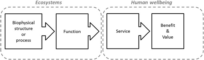
Links between ecosystems and human wellbeing. Modified from
Ecosystem functions are defined as the capacity of natural processes and components to provide goods and services that satisfy human needs, directly or indirectly; accordingly, they form a subset of ecological processes and ecosystem structures (
To date, different classification systems for ES are in use. They invariantly discriminate among provisioning services (the goods we obtain from ecosystems), regulating and maintenance services (the capacity of ecosystems to maintain a liveable environment), and cultural services (the non-material benefits). Well known provisioning services are water, timber, fish and agricultural products which are traded on markets. The supply of provisioning ecosystem services is heavily influenced by human inputs in the form of energy, labour and nutrient subsidies. Regulating services include the removal of pollutants from soil, air and water, or services which support crop production such as pollination and soil erosion control. They are directly dependent on the proper ecological functioning of ecosystems; they are not traded on markets so that their contribution to human well-being is more difficult to assess. Cultural services include, among others, nature-based recreation and tourism; they are, more than other services, essentially defined by human preferences.
A recent assessment of the potential consequences of climate change in Europe on several impact categories (i.e. agriculture, river floods, coastal areas, tourism and human health) has revealed large variations across regions in terms of damages and benefits (
A common approach to assess ES involves the use of land use and land cover (LULC) information in combination with other statistics and data to infer stocks and flows of ES generated by different ecosystems (
Considering both LULC projections and climate change (CC) scenarios, in principle, enables us to capture the main pressures acting on ecosystems and ES, thus enhancing the suitability of this approach to generate policy-relevant information. The establishment of the linkages among CC/LULC/ES, however, requires, amongst others, accurate considerations on issues related to the spatial and temporal scales characterising the involved processes; therefore, it can only be tackled in a stepwise approach – depending on the availability of data, tools and resources.
The focus of this study lies on regulating ecosystem services. This choice follows from differences among the main groups of ecosystem services: the delivery of regulating services, in fact, is tightly coupled to well-functioning ecosystems. This property makes regulating ES suitable examples for a first case study at a Pan-European scale.
This study provides an assessment on the possibility to establish relationships between CC, LULC and changes in ES (potential) supply, via bio-physical parameters that: (i) respond to climatic drivers; (ii) can be tied to ES with semi-quantitative or qualitative relationships, without the need of process-based models (which are beyond the scope of this study). This study is preliminary for a number of reasons: for instance, we only looked at impacts on three ES; additionally, due to the difficulties to assess the role of biodiversity as a service providing unit, we do not look at the impacts of climate and LULC changes on biodiversity, although we acknowledge that biodiversity is affected by changes in these drivers, and that biodiversity underpins ES. With these limitations in mind, our work quantifies, in relative terms, changes in ES provision across terrestrial ecosystems, induced by changes in both LULC and climate and, also, by changes in climate alone.
Materials and Methods
Overview
Every box in the cascade model of Fig.
In addition to selecting regulating services for being tightly coupled to well-functioning ecosystems, the final choice to include certain services was further influenced by the different models that were selected to establish the linkages between CC, LULC and ES:
- The Community Land Model (CLM) (
Oleson et al. 2010 ) provided the climate based scenarios of changes in ecosystems and ecosystem functioning. CLM examines the physical, chemical, and biological processes by which terrestrial ecosystems affect and are affected by climate. Some of the processes present within CLM are, for instance, vegetation and soil hydrology, energy fluxes, Carbon and Nitrogen cycling, and routing of runoff from rivers to oceans. Thus, CLM was the source of the bio-physical processes and structures as outlined in the cascade model (Fig.1 ). - The LUISA modelling platform (
Baranzelli et al. 2014 ) was used to spatially identify different ecosystems based on land cover and land use. Thus, LUISA was used to assess the actual ES provision, translating processes and functions into services (Fig.1 ).
The choice for these two models constrained the number of ecosystems and ecosystem services that could be covered in this assessment. As a result, we present the assessment for terrestrial ecosystems based on their capacity to deliver air quality regulation, soil retention (or soil erosion control) and water (quantity) regulation (capacity to regulate water flows which either supply or buffer water).
Fig.
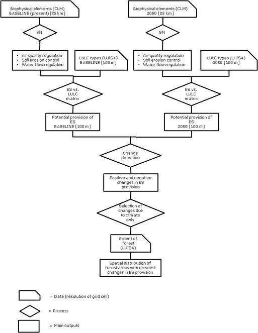
Main data, processes and outputs to estimate changes in ES provision. When relevant, sources of data are indicated within round brackets () and defined within the main text. The spatial resolution of information from LUISA and CLM is specified within square brackets []. BN = Bayesian Network; ES = Ecosystem Service(s); LULC = Land use / land cover
The next subsections provide a detailed description of the methods we followed.
ES choice and proxies
The ecosystem services (potential) supply was estimated using Bayesian Networks (BN), which enable us to model under uncertainty and to integrate different types of probabilistic information (
We used expert knowledge and available literature to select outputs from CLM which can be related to regulating ES (i.e. to define the nodes of the BN), as well as to define the relations between the selected CLM components and each specific ES (i.e. to define each ES model). The CLM outputs consisted of projections of terrestrial processes under the IPCC SRES A1B climate scenario, generated by three combinations of global and regional climate models (RCM). The CLM outputs have a spatial resolution of 25 km and a monthly temporal resolution, covering the period 1961 - 2099. We selected two 30-year non-overlapping periods to maximise the temporal overlap between CLM and LUISA frame: the present or 'baseline' (from 1991 to 2020), and the 2050 (from 2021 to 2050). For each period and CLM component, we then derived basic descriptive statistics such as minimum, maximum, average and standard deviation, pooling together the results from the three RCM. This information was used to reclassify the original CLM predicted values into relative scores between 0 and 1, and then to assign them their respective probabilities (see next paragraph).
As stated above, the selected CLM components represent different nodes of the BN. Conditional Probability Tables (CPT) were filled to reflect the distribution of states (i.e. their probability, p) resulting from each different climate model. More specifically, for each CLM output of interest, we applied Fisher’s intervals (
We built BNs for the following regulatory ES:
- Air quality regulation
- Soil erosion control
- Water flow regulation
This allowed us to detect and characterise how processes and functions underpinning the selected ES change over time. In particular, we assessed the projected changes for 2050, in relation to the baseline.
We selected 12 bio-physical variables from CLM, which we used as proxies for ecosystem functions or ecosystem processes, after establishing a positive or negative relationship with each relevant ecosystem service (Table
Bio-physical variables from the CLM (proxies for ecosystem functions, EF, or ecosystem processes, EP) and related ecosystem services (ES). Positive relationships between EF / EP and ES are indicated with ‘+’, negative relationships with ‘-’.
|
CLM component |
Ecosystem service and relationship |
|||
|
Description |
Name & Units |
|||
|
Leaf area index |
ELAI [m2/m2] |
Air quality regulation (+) |
||
|
Daily fire probability |
FIRE_P [0-1] |
Air quality regulation (-) |
||
|
Carbon in fine root |
FROOTC [gC/m2] |
Soil erosion control (+) |
||
|
Height of canopy top |
HTOP [m] |
Air quality regulation (+) |
||
|
Aquifer recharge rate |
QCHARGE [mm/s] |
Water flow regulation (+) |
||
|
Surface runoff |
QOVER [mm/s] |
Soil erosion control (-) |
||
|
Precipitation |
RAIN [mm/s] |
Air quality regulation (+) |
Water flow regulation (+) |
|
|
Ground evaporation |
QSOIL [mm/s] |
Water flow regulation (-) |
||
|
Canopy evaporation |
QVEGE [mm/s] |
Water flow regulation (-) |
||
|
Canopy transpiration |
QVEGT [mm/s] |
Water flow regulation (-) |
||
|
Total soil organic matter Carbon |
TOTSOMC [gC/m2] |
Soil erosion control (+) |
||
|
Water in the unconfined aquifer |
WA [gC/m2] |
Water flow regulation (+) |
||
Fig.
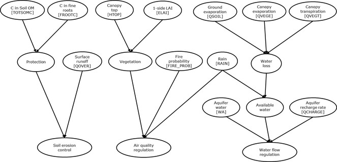
Schematic representation of the BN built for the assessment of the selected ES (Soil erosion control, Air quality regulation, Water flow regulation). Bio-physical components from the CLM are indicated within square brackets []. See Table
ES models
Here we present the ES models used within the BN, with reference to the relevant literature consulted to derive the relationships between the different model components.
Air quality regulation
The BN model to estimate air quality regulation included the contribution of three main elements: vegetation, rainfall and fire. The first two exerted a positive effect on air quality, whilst the last one a negative effect.
- Vegetation: Vegetation leaves absorb gaseous pollutants through their stomata, while particles are removed from the air by deposition onto leaves and branches (
Vos et al. 2013 ). Pollution removal is known to be positively related to tree cover and length of in-leaf season, and to vary with meteorological variables that affect tree transpiration and deposition velocities (Nowak et al. 2006 ). The contribution of vegetation was rendered by an additive effect of foliage and canopy height (ELAI and HTOP respectively, Table1 ). - Rainfall: Positive effects on removal capacity are also exerted by rainfall through wet deposition (
Cooter et al. 2013 ), although increased precipitation may also lead to reduced total removal via dry deposition (Nowak et al. 2006 ). In absence of information to quantify this effect, we accounted for this potential reduction by assigning a weight = 0.8 to the positive contribution of rainfall (RAIN, Table1 ). The implication of this choice are addressed in the 'Discussion'. - Fire: Wild or prescribed, fire can significantly degrade air quality by impairing visibility and releasing toxic by-products into the atmosphere. The susceptibility to open biomass burning events is likely to increase in Southern Europe, due to warmer and drier conditions predicted by climate change scenarios (
Giannakopoulos et al. 2009 ). Fire-related impacts and potential mitigation options are currently being investigated by several authors (e.g.Garcia-Hurtado et al. 2014 ,Sarigiannis et al. 2014 ). We accounted for the negative effect exerted by the fire by subtracting fire probability (FIRE_P, Table1 ) to the benefits derived from vegetation and rainfall.
In summary, the BN model for air quality regulation included five parent nodes (Fig.
Air quality regulation = Rain (w) + Vegetation control – Fire probability [Eq. 1]
Where:
- Rain (w) = 0.8 * RAIN;
- Vegetation control = Foliage (ELAI) + Canopy height (HTOP)
Soil erosion control
The BN model to estimate soil erosion control included the protective role of vegetation and soil organic content, and the negative effect of surface runoff, which causes erosion by water. We did not consider the potential contribution of specific support practices aimed at controlling erosion, such as policy implementation or voluntary measures, as this would require information we currently do not have. When we scored the contribution of different LULC types for their capacity to control soil erosion, however, we took into consideration that certain man-made elements can potentially provide a positive contribution to controlling erosion (
- Vegetation: We chose the amount of Carbon in fine roots (FROOTC, Table
1 ) to represent the protective role offered by vegetation. This choice was motivated by recent experiments investigating the role of root traits to reduce erosion rates by concentrated flow (Burylo et al. 2012 ). The results highlighted that the potential to reduce erosion was negatively correlated to root diameter, and positively correlated to the percentage of fine roots. - Soil organic matter: In addition to fine roots, we also included soil organic matter (TOTSOMC, Table
1 ) as a protective component; greater organic matter into the soil, in fact, provides better structural and water-holding qualities (Lal 1994 ). - Surface runoff: We used surface runoff (QOVER, Table
1 ) to represent the erosion caused by water flow (Toy et al. 2002 ).
The estimated soil erosion control resulted from subtracting the effect of surface runoff to the estimated protection obtained from fine roots and soil organic matter.
In summary, the BN model for soil erosion control included four parent nodes (Fig.
Erosion Control = Protection – Surface runoff [Eq. 2]
Where:
- Protection = Vegetation (FROOTC)+ Soil organic matter (TOTSOMC)
- Surface runoff = QOVER
Water flow regulation
The BN model to estimate water flow regulation included the contribution of four components of the hydrological cycle, making up the surface and groundwater: rainfall, water loss (from evaporation and transpiration), water in the unconfined aquifer and aquifer recharge rate. We chose these variables as they might be directly affected by changing climate, for instance as a result of changes in temperature or rainfall patterns (
- Surface water: We chose precipitation amount (RAIN, Table
1 ) minus water loss, to represent the potential source of surface water (Bagstad et al. 2011 ). We represented water loss by summing the contribution of ground evaporation (QSOIL, Table1 ) and evapotranspiration (canopy evaporation and canopy transpiration, QVEGE and QVEGT respectively, Table1 ) (Pistocchi et al. 2008 ,Vigerstol and Aukema 2011 ). - Ground water: We used water in the unconfined aquifer and aquifer recharge rate (WA and QCHARGE respectively, Table
1 ) to represent groundwater (Jujnovsky et al. 2012 ).
Scores from the BN model for water supply ranged potentially between -1 and +3 (Fig.
Water supply = Water in the unconfined aquifer + Aquifer recharge rate + Available water [Eq. 3]
Where:
- Water in the unconfined aquifer = WA
- Aquifer recharge rate = QCHARGE
- Available water = RAIN – Water loss;
- Water loss = Ground evaporation (QSOIL) + Canopy evaporation (QVEGE)+ Canopy transpiration (QVEGT)
LULC contribution to ES delivery
The (climate-based) results from the BN were then weighted according to the underlying land use and land cover (LULC) type, to better reflect the differences in the relative contribution of LULC types to support ES provision. We followed the ‘ES potential matrix’ method provided in
- The rounded up average from the scores of
Burkhard et al. (2014) was taken, when a LUISA LULC type included more than one CORINE land cover type; - All scores were rescaled to the 0.0 to 1.0 range.
Fig.
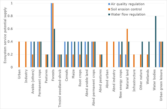
Relative capacity (y-axis) of LULC types (x-axis) to supplying regulating ES (air quality regulation, soil erosion control and water flow regulation). LULC types are defined as in LUISA (
Assessing relative changes in ES provision
To highlight areas where climate change is estimated to induce changes in the CLM inputs, we first extracted the percent change between 2050 and the baseline for each bio-physical parameter used within the BN model. We expected that major changes in the BN inputs would also propagate through the relevant ES.
Subsequently, following the ES per LULC matrix, we assessed the potential supply of ES, for the baseline and the 2050 scenario. From these two assessments we calculated the percent change over time and across geographical space, for each ES. The use of percentage also allowed us to compare changes in ES supply across ES see also
Further to this assessment, we extracted all areas where LULC was predicted to remain the same over time and we quantified the changes in ES provision, solely due to changing climatic conditions. This refinement allowed us to quantify the ES climate-induced changes in relation to those caused by changes in both drivers (LULC and climate).
Lastly, we highlighted the greatest positive and negative changes in ES provision occurring in forests throughout Europe.
Results
Changes in the bio-physical variables supporting ecosystem processes
Climate change following the model predictions for the A1B scenario is expected to have a profound impact on the different ecological functions used in this study to derive ecosystem services (Fig.
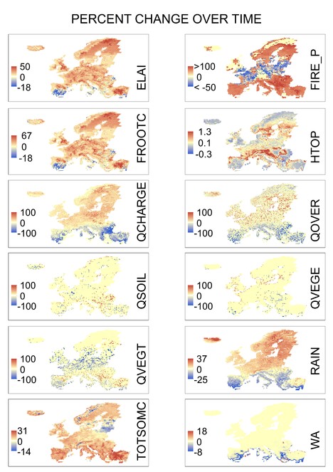
CLM model outcomes showing climate-induced percent change between 2050 and the baseline, for the bio-physical variables used as inputs of the ES-BN models. See Table 1 for a definition of the variable names. The magnitude and spatial extent of change can be categorised in five main patterns: (1) Great magnitude of change, widely spread across the study area (FIRE_P and QCHARGE); (2) Great magnitude of change for very limited regions, and the majority of the regions laying around small changes (QOVER, QSOIL, QVEGE and QVEGT); (3) Small magnitude of change, but widely spread across the study area (e.g. ELAI, FROOTC, RAIN, TOTSOMC); (4) Small magnitude of change, spatially localised (WA); (5) Very small change, but widely spread (HTOP). Distribution maps are displayed using non-projected Geographic Reference System (WGS84 Datum).
The expected plant productivity, in general, will increase across Europe. This is visible from the expected changes in exposed one-side leaf area index (ELAI), and in the root biomass with increasing fine root carbon (FROOTC) and total soil organic matter carbon (TOTSOMC). The magnitude of these changes is relatively small, but widely spread across the study area.
Aquifer recharge rates (QCHARGE) and the daily fire probability (FIRE_P) are expected to exhibit substantial changes in both directions (positive and negative), widely spread across the study area. Fire probability is expected to increase in north and south Europe while decreases are foreseen in the areas in between. Aquifer recharge rates are expected to fall in the Mediterranean, following the altered patterns of rainfall (RAIN).
Four functions, surface runoff (QCOVER), ground evaporation (QSOIL), canopy evaporation (QVEGE) and canopy transpiration (QVEGT) are expected to change in both directions for very limited regions, while for the majority of the regions small changes are foreseen.
Water in the unconfined aquifer (WA) is expected to undergo small and spatially localised changes while the canopy top (HTOP) will slightly change across Europe.
Changes in ES provision due to potential changes in LULC and climate
The next three assessments quantify the relative provision of ES for the baseline and for 2050, under a scenario of changes potentially occurring both drivers (LULC and climate).
Air quality regulation
Fig.
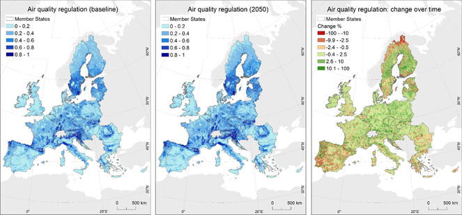
Air quality regulation for baseline, 2050 and as a percent change over time (2050 vs. baseline). For the baseline and the 2050 maps, classes represent equal intervals over the range of rendered predictions; for the percent change over time, the visual representation reflects the distribution of the values. Maps are displayed using the Projected Reference System LAEA. See main text for additional details.
The percent change between 2050 and the baseline showed that most of the values were bound by the ±10% change with very few values towards the extreme ends (mean = 1.2 and SD = 11.6). The visual representation, therefore, was chosen to reflect this distribution. Areas of greatest negative change were mainly located in the EU-28 Scandinavian countries, in the Iberian Peninsula and on the South-East part of Europe.
Fig.
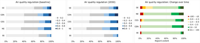
From left to right, air quality regulation for the baseline, the 2050 and as percent change over time. The scores are shown in relation to the percent extent of five European regions, defined after grouping the 28 Member States (MS) according to their climatic characteristics (
Soil erosion control
Fig.
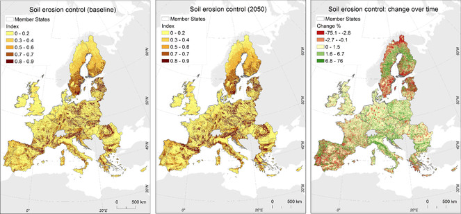
Soil erosion control for the baseline, the 2050 and as a percent change over time (2050 vs. baseline). For the baseline and the 2050 maps, classes represent equal intervals over the range of rendered predictions; for the percent change over time, the visual representation reflects the distribution of the values. Maps are displayed using the Projected Reference System LAEA. See main text for additional details.
The percent change between 2050 and the baseline showed that most of the values were within -2.8% and +6.8% change, with very few values towards the extreme ends (mean = 1.2 and SD = 13.4). The visual representation, therefore, was chosen to reflect this distribution. Extended areas of greatest negative change were located both in North and South Europe; in both regions, however, there were also noticeable areas of positive change.
Fig.
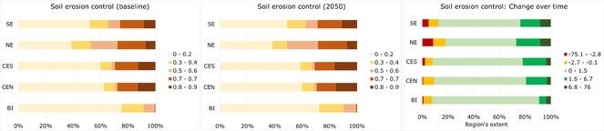
From left to right, soil erosion control for the baseline, the 2050 and as percent change over time. The scores are shown in relation to the percent extent of five European regions, defined after grouping the 28 Member States (MS) according to their climatic characteristics (
The percent change over time (2050 vs. baseline) revealed that across all five regions the vast majority of their area was characterised by a little positive increase in the capacity of controlling soil erosion (although with similar SD, this effect is likely to be non-significant). Interestingly, North Europe was characterised by the greatest extent of both positive and negative changes (Fig.
Water flow regulation
Fig.
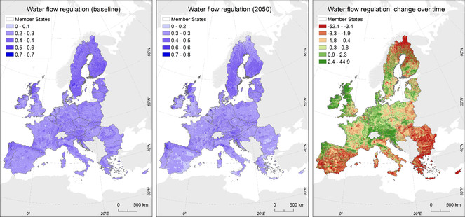
Water flow regulation for the baseline, the 2050 and as a percent change over time (2050 vs. baseline). For the baseline and the 2050 maps, classes represent equal intervals over the range of rendered predictions; for the percent change over time, the visual representation reflects the distribution of the values. Maps are displayed using the Projected Reference System LAEA. See main text for additional details.
The map for the baseline water flow regulation did not show a spatial pattern in the distribution of scores, whilst the 2050 prediction showed some regions with greater capacity of regulating water flow (e.g. Northern part of the British Isles, vast areas in the EU-28 Scandinavian countries, Northern part of The Netherland and of Portugal, to give a few examples).
The percent change between 2050 and the baseline showed that most of the values were within -3.4% and +2.4% change, with very few values towards the extreme ends (mean = -0.4 and SD = 6.3). The visual representation, therefore, was chosen to reflect this distribution. Extended areas of greatest negative change were located in the Northern-most part of the EU-28 Scandinavian countries as well as in the South-East part of Europe and Iberian Peninsula. Areas of positive change were visible in the Southern part of Central Europe, in the Northern part of the British Isles and of Portugal.
Fig.
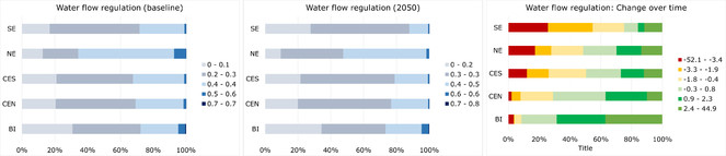
From left to right, water flow regulation for the baseline, the 2050 and as percent change over time. The scores are shown in relation to the percent extent of five European regions, defined after grouping the 28 Member States (MS) according to their climatic characteristics (
The percent change over time (2050 vs. baseline) showed that the largest extent of negative change was recorded in South Europe, immediately followed by North Europe. The eastern part of Central Europe was characterised by a rather homogenous change cross all six classes, whilst in the British Isles we observed the largest extent of positive change (Fig.
Changes in ES provision due to changes in climate alone
Figs
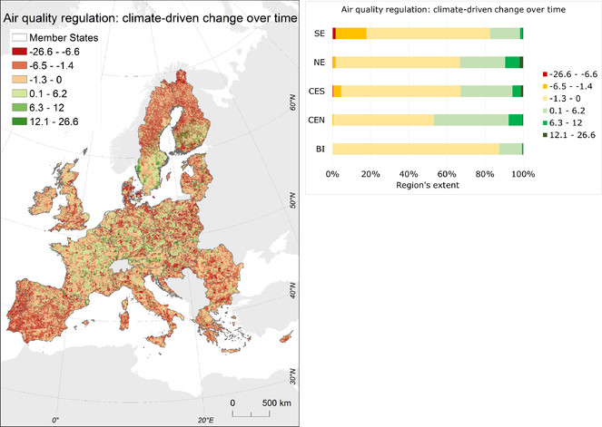
Change in air quality regulation over time (2050 vs. baseline), in areas where LULC was predicted to remain unchanged. Areas mapped in dark red indicate largest percent decrease, areas mapped in dark green indicate the largest percent increase. The bar chart shows the change as a relative extent percent, for five European regions defined after grouping the 28 Member States according to their climatic characteristics (
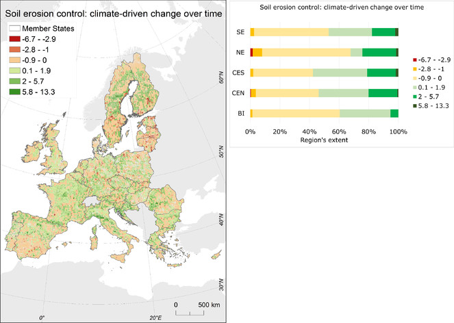
Change in soil erosion control over time (2050 vs. baseline), in areas where LULC was predicted to remain the same. Areas mapped in dark red indicate largest percent decrease, areas mapped in dark green indicate the largest percent increase. The bar chart shows the change as a relative extent percent, for five European regions defined after grouping the 28 Member States according to their climatic characteristics (
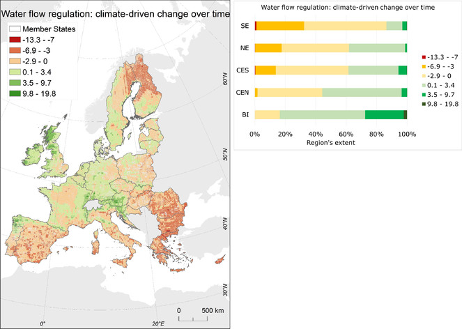
Change in water flow regulation over time (2050 vs. baseline), in areas where LULC was predicted to remain the same. Areas mapped in dark red indicate largest percent decrease, areas mapped in dark green indicate the largest percent increase. The bar chart shows the change as a relative extent percent, for five European regions defined after grouping the 28 Member States according to their climatic characteristics (
Compared to Figs
In general, it is noticeable that the magnitude of change does not include extreme values: ad-hoc inspections revealed in fact that the greatest changes in absolute values were often caused by land conversion from one class to another one: for instance, if an area was predicted to undergo conversion from forest to arable land between the baseline and 2050, the score for the capacity of the underlying ecosystems to control soil erosion would change from 1 (forest) to 0.2 (arable land) (Fig.
Air quality regulation
Fig.
Soil erosion control
Fig.
Water flow regulation
Fig.
Changes in forest areas
Fig.
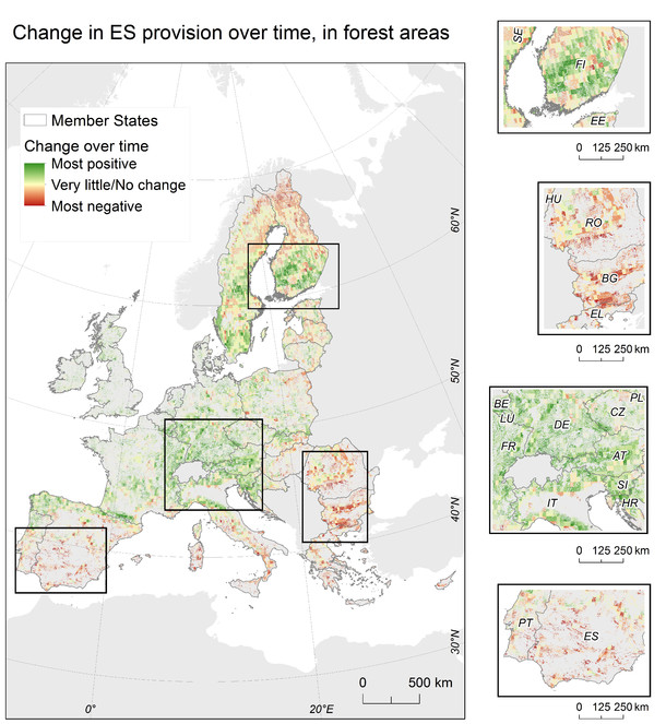
Change in ecosystem service provision over time (2050 vs. baseline) in forest areas over EU-28 (left) and close-up examples (right). Dark shades of green correspond to great positive change, and indicate areas with the greatest increase in ES provision, dark shades of red correspond to great negative change and indicate areas with the greatest decrease in ES provision. Maps are displayed using the Projected Reference System LAEA.
Discussion
With this study we tested the feasibility to link climate change and changes in land cover and land use to show changes in the supply of three regulating ecosystem services, across terrestrial ecosystems. Additionally, we identified areas where greatest positive and negative changes are expected, in a given ecosystem (here represented by a LULC type).
Main highlights
A few points can be highlighted from our work:
- Mapping the predicted changes in the bio-physical functions underpinning the three regulating ES, helped us understand some of the predicted changes in the dependent ES. For instance, inspecting the changes in the components of water flow regulation (the ES with the predicted greatest negative change), showed noticeable changes for several of them: 'Aquifer recharge rate' (QCHARGE) above all, with great magnitude of change (positive and negative), widely spread across Europe; ‘Water in the unconfined aquifer' (WA), with localised but important changes in the Southern part of Europe; and ‘Precipitation’ (RAIN), characterised by small magnitude of change, but widely spread across Europe.
- Inspecting the changes in LULC, revealed potential major effects on ES supply.
- We considered climate change and LULC as additive effects. But the changes in both drivers are likely to lead to more complex effects than expected by their additions (
Elmhagen et al. 2015 ). Similarly, the combined increase of temperature, rainfall and CO2 is likely to lead to complex interactions and feedbacks: for instance, increased CO2 reduces stomatal conductance, which reduces transpiration and counteracts a potential increase in evapotranspiration caused by warming (Kløve et al. 2014 ).
The role of local management strategies
We performed the analysis at the extent of EU-28, using climate data with a spatial resolution of ca. 25 km and LULC information with a much finer spatial resolution (100 m). We did not include local management strategies which might be in place in certain areas, as this information cannot be readily integrated into our models and would require arbitrary decisions on conversion factors and weights, which could have a significant influence on the predictions. Our outcome, therefore, offers an overview of what can be expected across EU-28. Hence, patterns emerging from our work should be compared with, and complemented by, the increasing number of studies that are becoming available both at European and local scale:
- At European scale for instance,
Panagos et al. (2015b) recently proposed a modified version of the RUSLE model (RUSLE2015), where cover-management factor (Panagos et al. 2015a ) and support practices in arable land are incorporated into their model, to estimate soil loss rates by water for the reference year 2010. Despite our approaches and input variables are different, the predicted outcomes show some similarities: for instance, general low rates of soil erosion throughout most Scandinavian countries and continental Europe predicted by the RUSLE2015 model, and relatively high potential for erosion control resulting from our assessment. - At local scale for instance,
Bangash et al. (2013) found that under the A2 and B1 CC scenarios (IPCC 2000 ), soil erosion control and water provision along the Llobregat river basin (Spain) are going to be negatively affected; this is likely due to the increasing frequency of flood and drought events predicted across the Iberian Peninsula.
Refining the European-wide results with local scale information would allow us to account for processes that vary at very local scale, such as the effects of pressure on hydrology. Local scale information would also allow us to evaluate the combined effects of different mitigation strategies:
Kiedrzyńska et al. (2015) , for instance, showed how effective management of river floodplains can be used to mitigate against the predicted increase in flood events; they highlighted a combination of different mitigation strategies, involving modelling, land use management for better water retention capacity, and infrastructure. It is also widely recognised, however, that more information is needed on several mechanisms at the basis of ecosystem functioning (and hence, ES provision), such as groundwater recharge (Kløve et al. 2014 ).
Changes in ES supply in forests
When assessing the results from changes induced by climate-only, we chose forests as an ES provider as they support the provision of many ES, and certainly of all the ES assessed here (Fig.
- Due to constraints on the input data, we only considered a broad definition of forest. A differentiation between forest types (e.g. broad-leaves, coniferous, etc.) is not currently contemplated by LUISA. A workaround, which however was not feasible with the available resources, is to use the CORINE classification to differentiate between different types of forest, and projected climate change to find the closest analogous climate for a set of representative woody species. This approach, however, is poor for at least two reasons: (i) it assumes that the closest suitable climate will be within species’ dispersal capacity, contradicting current literature (
Ohlemüller et al. 2006a ,Ohlemüller et al. 2006b ) ; and (ii) it does not account for human interventions reacting to climate change or policy directives. - Forests are expected to increase under the climatic projections of the next decades, for instance due to increased availability of CO2 and, at least in Europe, as a consequence of agricultural land-abandonment and policy strategies. Yet, an increased in forest extent does not necessarily imply increased biodiversity (particularly for mono-specific forest plantations grown mainly for biomass production). In addition, evidence shows that several climate change projections are expected to produce unsuitable conditions for many species, and closest climate analogues beyond species’ dispersal capacity (
Ohlemüller et al. 2006a ,Ohlemüller et al. 2006b ). These two elements do not support the idea of stable forest communities anymore, implying the need of societal interventions to ensure forest’s viability. Therefore, the increased in ES supply provided by a certain ecosystem, might only apply to a few ES and would lead to biased conclusion if used as the only criterion to assess the effects of CC and LULC changes.
Final remarks
Some final remarks, but not of less importance, are on the assumptions and limitations of our method:
- We have only considered one CC scenario (A1B) due to constraints on the input data. Our results, therefore, offer two snapshots in time (baseline and 2050 projections) of a very complex and wider reality.
- We have captured some of the uncertainty related to CC projections by considering three different Regional Climate Models and by accounting for their differences while building the Bayesian Network, as well as when summarising their predictions. But the complexity of the subject would as well grant an examination of the uncertainty related to each of its components, from the input data to the processes and, where applicable, choice of weights, from the existing knowledge to the available tools. As noticed for instance by
Grêt-Regamey et al. (2013) , however, such an analysis would require a separate trans-disciplinary process, to be really informative. - We have assumed the same scaling properties between the ES considered in our study: as such, a unit change in one ecosystem was weighted equally when deriving the quantile split. In absence of sufficient bio-physical evidence we lack the necessary information to support different choices.
- We have assumed that any perturbation will have the same effect on the system: in other words, we have not included ‘tipping points’, i.e. critical thresholds at which a tiny perturbation can qualitatively alter the state or development of a system (
Lenton et al. 2008 ). Incorporating this information remains a major research challenge, already highlighted, for instance, byCiscar Martinez et al. (2014) . Yet it is a key element to determine planetary boundaries, which are defined upstream the tipping point to buffer uncertainty, and should be used to guide human choices towards sustainable development (Steffen et al. 2015 ).
Conclusions
This work represents a preliminary spatially explicit assessment of the CC impacts on ES provision. As anticipated by
Despite these limitations, our work has also some highlights:
- To our knowledge, this is the first spatially explicit example of an EU-wide assessment linking CC, LULC and ES. It brings together scientifically accepted models (e.g. CLM and LUISA) and the latest tools for ES-LULC mapping (e.g. the ES potential matrix), to derive the potential changes in ES provisions, caused by CC alone, as well as by the combined change in climate and LULC.
- Linking climate and LULC models enabled us to produce results at a spatial resolution finer than what would be obtained using climate models only. This is important not only to better represent variation and processes acting at local scale, but also to better inform local scale interventions.
- This work is based on semi-automated procedures which can be routinely repeated as more (or better) information becomes available. This is particularly important given that this area of research is expanding, and can therefore provide evidence-based scientific and technical support to the EU policy cycle.
In addition to these methodological highlights, the results allow us to draw at least two general conclusions:
- Positive and negative changes are spatially distributed, with a tendency for negative changes to be distributed at the periphery of the study area (i.e. mainly in the northern and southern areas), and positive changes to be distributed towards the central parts. This is particularly noticeable when looking at the changes affecting water flow regulation. This general pattern is probably a consequence of climatic conditions being already at the extreme of their reference range in the northern and southern areas.
- LULC change is a stronger driver than climate change on the provision of ES: this has important implications as it suggests that the impacts of climate change can be mitigated through adaptive ecosystem management.
Acknowledgements
We thank I. Gonzalez-Aparicio for her support in accessing the CLM outputs. This study was part of the GAP PESETA project which received funding from the Directorate-General Climate Action (contract number 33371).
Hosting institution
European Commission, Joint Research Centre (Ispra, Italy).
Author contributions
Maes J. conceived the idea; Baranzelli C. and Lavalle C. provided access to LUISA land use and land cover data; Cescatti A. provided access to the CLM outputs; Polce C. designed the BN models and analysed the data. Maes J. and Polce C. prepared the draft manuscript and all authors contributed to its revision.
Conflicts of interest
The authors declare no conflicts of interest.
References
- ARIES: Artifical Intelligence for Ecosystem Services: A guide to models and data, version 1.0.The ARIES Consortium,128pp. URL: http://aries.integratedmodelling.org/wp-content/uploads/2016/03/ARIESModelingGuide1.0.pdf
- Ecosystem services in Mediterranean river basin: Climate change impact on water provisioning and erosion control.Science of The Total Environment458-460:246‑255. https://doi.org/10.1016/j.scitotenv.2013.04.025
- The Reference Scenario in the LUISA platform - Updated configuration 2014 - Towards a Common Baseline Scenario for EC Impact Assessment procedures.Publications Office of the European Union,45pp. [ISBN978-92-79-44702-0] https://doi.org/10.2788/85104
- Contribution of ecosystem services to air quality and climate change mitigation policies: The case of urban forests in Barcelona, Spain.Ambio43(4):466‑479. https://doi.org/10.1007/s13280-014-0507-x
- Bayesian networks in environmental and resource management.Integrated Environmental Assessment and Management8(3):418‑429. https://doi.org/10.1002/ieam.1327
- Guidance manual on value transfer methods for ecosystem services. United Nations Environment Programme.Publishing Services Section, UNON,Nairobi, Kenya,77pp. [ISBN978-92-807-3362-4]
- Using Meta-Analysis and GIS for Value Transfer and Scaling Up: Valuing Climate Change Induced Losses of European Wetlands.Environmental and Resource Economics52(3):395‑413. https://doi.org/10.1007/s10640-011-9535-1
- Ecosystem Service Potentials, Flows and Demands - Concepts for Spatial Localisation, Indication and Quantification.Landscape Online34:1‑32. https://doi.org/10.3097/LO.201434
- Mapping ecosystem service supply, demand and budgets.Ecological Indicators21:17‑29. https://doi.org/10.1016/j.ecolind.2011.06.019
- Plant root traits affecting the resistance of soils to concentrated flow erosion.Earth Surface Processes and Landforms37(14):1463‑1470. https://doi.org/10.1002/esp.3248
- Planning improvements in natural resources management: Guidelines for using Bayesian networks to support the planning and management of development programmes in the water sector and beyond.CEH,Wallingford,132pp. [ISBN0 903741 00 9]
- Modeling land use decisions with Bayesian networks: Spatially explicit analysis of driving forces on land use change.Environmental Modelling & Software52:222‑233. https://doi.org/10.1016/j.envsoft.2013.10.014
- Cerqueira Y, Navarro LM, Maes J, Marta-Pedroso C, Pradinho Honrado J, Pereira HM (2015) Ecosystem Services: The Opportunities of Rewilding in Europe. In: Pereira HM, Navarro LM (Eds) Rewilding European Landscapes.Springer,17pp. [ISBN978-3-319-12039-3 (Online)]. https://doi.org/10.1007/978-3-319-12039-3_3
- Physical and economic consequences of climate change in Europe.Proceedings of the National Academy of Sciences of the United States of America108(7):2678‑2683. https://doi.org/10.1073/pnas.1011612108
- Climate Impacts in Europe. The JRC PESETA II Project.Publications Office of the European Union,155pp. [ISBN978-92-79-36833-2] https://doi.org/10.2791/7409
- The role of the atmosphere in the provision of ecosystem services.Science of The Total Environment448:197‑208. https://doi.org/10.1016/j.scitotenv.2012.07.077
- Functions of Nature: Evaluation of Nature in Environmental Planning, Management and Decision Making.Wolters-Noordhoff,Groningen, NL,xviii + 315pp. [ISBN1475-3057] https://doi.org/10.1017/S0032247400023779
- The 2015 ageing report - Economic and budgetary projections for the 28 EU Member States (2013-2060).Publications Office of the European Union,424pp. [ISBN1725-3217] https://doi.org/10.2765/877631
- Interacting effects of change in climate, human population, land use, and water use on biodiversity and ecosystem services.Ecology and Society20(1):23. https://doi.org/10.5751/es-07145-200123
- Climate change in Europe. 1. Impact on terrestrial ecosystems and biodiversity. A review (Reprinted).Agronomy for Sustainable Development29(3):409‑421. https://doi.org/10.1051/agro:2008066
- On Grouping for Maximum Homogeneity.Journal of the American Statistical Association53(284):789‑798. https://doi.org/10.1080/01621459.1958.10501479
- Atmospheric PM and volatile organic compounds released from Mediterranean shrubland wildfires.Atmospheric Environment89:85‑92. https://doi.org/10.1016/j.atmosenv.2014.02.016
- Climatic changes and associated impacts in the Mediterranean resulting from a 2 °C global warming.Global and Planetary Change68(3):209‑224. https://doi.org/10.1016/j.gloplacha.2009.06.001
- Integrating Expert Knowledge into Mapping Ecosystem Services Trade-offs for Sustainable Forest Management.Ecology and Society18(3). https://doi.org/10.5751/es-05800-180334
- Quantifying and mapping the human appropriation of net primary production in earth's terrestrial ecosystems.Proceedings of the National Academy of Sciences104(31):12942‑12947. https://doi.org/10.1073/pnas.0704243104
- Haines-Young R, Potschin M (2010) The links between biodiversity, ecosystem services and human well-being. In: Raffaelli D, Frid (Hg.) C (Eds) Ecosystem Ecology: a new synthesis. BES Ecological Reviews Series. Cambridge: Cambridge University Press (iE).
- The Economics of Ecosystems and Biodiversity. The quantitative Assessment. Final Report to the United Nations Environment Programme.Full text PDF,243pp. URL: https://www.researchgate.net/publication/241870310_The_Economics_of_Ecosystems_and_Biodiversity_the_Quantitative_Assessment
- Emissions Scenarios. Summary for Policymakers.Intergovernmental Panel on Climate Change,27pp. URL: https://www.ipcc.ch/pdf/special-reports/spm/sres-en.pdf [ISBN92-9169-113-5]
- Assessment of Water Supply as an Ecosystem Service in a Rural-Urban Watershed in Southwestern Mexico City.Environmental management49(3):690‑702. https://doi.org/10.1007/s00267-011-9804-3
- Sustainable floodplain management for flood prevention and water quality improvement.Natural Hazards76(2):955‑977. https://doi.org/10.1007/s11069-014-1529-1
- Climate change impacts on groundwater and dependent ecosystems.Journal of Hydrology518:250‑266. https://doi.org/10.1016/j.jhydrol.2013.06.037
- Global human appropriation of net primary production doubled in the 20th century.Proceedings of the National Academy of Sciences110(25):10324‑10329. https://doi.org/10.1073/pnas.1211349110
- Soil erosion research methods.CRC Press,352pp. URL: http://tinyurl.com/lmhxwth [ISBN1884015093]
- A review of Bayesian belief networks in ecosystem service modelling.Environmental Modelling and Software46:1‑11. https://doi.org/10.1016/j.envsoft.2013.03.011
- Tipping elements in the Earth's climate system.Proceedings of the National Academy of Sciences105(6):1786‑1793. https://doi.org/10.1073/pnas.0705414105
- Assessment of coastal protection as an ecosystem service in Europe.Ecological Indicators30:205‑217. https://doi.org/10.1016/j.ecolind.2013.02.013
- Mainstreaming ecosystem services into EU policy.Current Opinion in Environmental Sustainability5(1):128‑134. https://doi.org/10.1016/j.cosust.2013.01.002
- Mapping ecosystem services for policy support and decision making in the European Union.Ecosystem Services1(1):31‑39. https://doi.org/10.1016/j.ecoser.2012.06.004
- Trends in ecosystems and ecosystem services in the European Union between 2000 and 2010.Publications Office of the European Union,138pp. [ISBN978-92-79-46206-1] https://doi.org/10.2788/341839
- Trade-offs across value-domains in ecosystem services assessment.Ecological Indicators37, Part A:220‑228. https://doi.org/10.1016/j.ecolind.2013.03.003
- Ecosystems and Human Well-being: Synthesis.Island Press,Washington, DC,155pp.
- Dynamic Bayesian Networks as a Decision Support tool for assessing Climate Change impacts on highly stressed groundwater systems.Journal of Hydrology479:113‑129. https://doi.org/10.1016/j.jhydrol.2012.11.038
- Air pollution removal by urban trees and shrubs in the United States.Urban forestry & urban greening4(3):115‑123. https://doi.org/10.1016/j.ufug.2006.01.007
- Quantifying components of risk for European woody species under climate change.Global Change Biology12(9):1788‑1799. https://doi.org/10.1111/j.1365-2486.2006.01231.x
- Towards European climate risk surfaces: the extent and distribution of analogous and non-analogous climates 1931–2100.Global Ecology and Biogeography15(4):395‑405. https://doi.org/10.1111/j.1466-822X.2006.00245.x
- Technical Description of version 4.0 of the Community Land Model (CLM).National Center for Atmospheric Research,Boulder, CO,257pp. [ISBN2153-2397]
- Estimating the soil erosion cover-management factor at the European scale.Land Use Policy48:38‑50. https://doi.org/10.1016/j.landusepol.2015.05.021
- The new assessment of soil loss by water erosion in Europe.Environmental Science & Policy54:438‑447. https://doi.org/10.1016/j.envsci.2015.08.012
- Mapping cultural ecosystem services: A framework to assess the potential for outdoor recreation across the EU.Ecological Indicators45:371‑385. https://doi.org/10.1016/j.ecolind.2014.04.018
- A simplified parameterization of the monthly topsoil water budget.Water Resources Research44(12):1‑21. https://doi.org/10.1029/2007wr006603
- The role of benefit transfer in ecosystem service valuation.Ecological Economics115:51‑58. https://doi.org/10.1016/j.ecolecon.2014.02.018
- Bayesian belief modeling of climate change impacts for informing regional adaptation options.Environ. Model. Softw.44:113‑121. https://doi.org/10.1016/j.envsoft.2012.07.008
- Total exposure to airborne particulate matter in cities: The effect of biomass combustion.Science of The Total Environment493:795‑805. https://doi.org/10.1016/j.scitotenv.2014.06.055
- A new map of global urban extent from MODIS satellite data.Environmental Research Letters4:1‑11. https://doi.org/10.1088/1748-9326/4/4/044003
- Ecology: Ecosystem service supply and vulnerability to global change in Europe.Science310(5752):1333‑1337. https://doi.org/10.1126/science.1115233
- Planetary boundaries: Guiding human development on a changing planet.Science347(6223):736‑12. https://doi.org/10.1126/science.1259855
- The Economics of Ecosystems and Biodiversity: Ecological and Economic Foundations.Routledge,Abingdon and New York,456pp. [ISBN978-0415501088]
- Soil erosion: processes, prediction, measurement, and control.John Wiley & Sons,352pp. [ISBN0471383694]
- The TEEB Valuation Database – a searchable database of 1310 estimates of monetary values of ecosystem services.Foundation for Sustainable Development. URL: http://www.fsd.nl/esp/80763/5/0/50
- A comparison of tools for modeling freshwater ecosystem services.Journal of Environmental Management92:2403‑2409. https://doi.org/10.1016/j.jenvman.2011.06.040
- Improving local air quality in cities: To tree or not to tree?Environmental Pollution183:113‑122. https://doi.org/10.1016/j.envpol.2012.10.021
- Predicting impacts of increased CO 2 and climate change on the water cycle and water quality in the semiarid James River Basin of the Midwestern USA.Science of The Total Environment430:150‑160. https://doi.org/10.1016/j.scitotenv.2012.04.058
- ESTIMAP: A GIS-based model to map ecosystem services in the European Union.Annali di Botanica4:1‑7. URL: http://ojs.uniroma1.it/index.php/Annalidibotanica/article/view/11807/11810
Supplementary materials
Example of a simple Bayesian Network and brief description of its main components.
Key between LUISA (Baranzelli et al., 2014) and CORINE LULC types, and scores for the potential contribution of each LULC type to provide relevant ES. Scores are based on the ES potential matrix by Burkhard et al. (2014), after appropriate rescaling. See main text for additional details.
Regional classification of the 28 EU Member States, updated from Ciscar et al. (2011).