|
One Ecosystem :
Review Article
|
|
Corresponding author:
Academic editor: Benjamin Burkhard
Received: 24 Mar 2016 | Accepted: 20 Jun 2016 | Published: 27 Jun 2016
© 2016 Anne Thessen
This is an open access article distributed under the terms of the Creative Commons Attribution License (CC BY 4.0), which permits unrestricted use, distribution, and reproduction in any medium, provided the original author and source are credited.
Citation:
Thessen A (2016) Adoption of Machine Learning Techniques in Ecology and Earth Science. One Ecosystem 1: e8621. https://doi.org/10.3897/oneeco.1.e8621
|
|
Abstract
Background
The natural sciences, such as ecology and earth science, study complex interactions between biotic and abiotic systems in order to understand and make predictions. Machine-learning-based methods have an advantage over traditional statistical methods in studying these systems because the former do not impose unrealistic assumptions (such as linearity), are capable of inferring missing data, and can reduce long-term expert annotation burden. Thus, a wider adoption of machine learning methods in ecology and earth science has the potential to greatly accelerate the pace and quality of science. Despite these advantages, the full potential of machine learning techniques in ecology and earth science has not be fully realized.
New information
This is largely due to 1) a lack of communication and collaboration between the machine learning research community and natural scientists, 2) a lack of communication about successful applications of machine learning in the natural sciences, 3) difficulty in validating machine learning models, and 4) the absence of machine learning techniques in a natural science education. These impediments can be overcome through financial support for collaborative work and the development of graduate-level educational materials about machine learning. Natural scientists who have not yet used machine learning methods can be introduced to these techniques through Random Forest, a method that is easy to implement and performs well. This manuscript will 1) briefly describe several popular machine learning tasks and techniques and their application to ecology and earth science, 2) discuss the limitations of machine learning, 3) discuss why ML methods are underutilized in natural science, and 4) propose solutions for barriers preventing wider ML adoption.
Keywords
ecology, machine learning, earth science, statistical learning
Introduction
Machine Learning (ML) is a discipline of computer science that develops dynamic algorithms capable of data-driven decisions, in contrast to models that follow static programming instructions. The very first mention of ‘machine learning’ in the literature occurred in 1930 and use of the term has been growing steadily since 1980 (Fig.
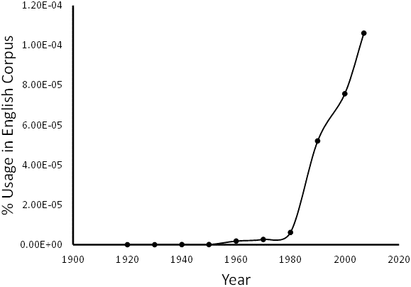
Use of the phrase ‘machine learning’ in the Google Books Ngram Viewer: This plot shows the use of the phrase ‘machine learning’ by decade as percentage of total words in the Google English Corpus. http://books.google.com/ngrams
The advantage of ML over traditional statistical techniques, especially in earth science and ecology, is the ability to model highly dimensional and non-linear data with complex interactions and missing values (
The exact division between ML methods and traditional statistical techniques is not always clear and ML methods are not always better than traditional statistics. For example, a system may not be linear, but a linear approximation of that system may still yield the best predictor. The exact method(s) must be chosen based on the problem at hand. A meta approach that considers the results of multiple algorithms may be best. This manuscript will discuss four types of ML tasks and seven important limitations of ML methods. These tasks and limitations will be related to six types of ML techniques and their relative strengths and weaknesses in ecology and earth science will be discussed. Specific applications of ML in ecology and earth science will be briefly reviewed with the reasons ML methods are underutilized in natural sciences. Potential solutions will be proposed.
Background
The basic premise of ML is that a machine (i.e., algorithm or model) is able to make new predictions based on data. The basic technique behind all ML methods is an iterative combination of statistics and error minimization or reward maximization, applied and combined in varying degrees. Many ML algorithms iteratively check all or a very high number of possible outcomes to find the best result, with “best” defined by the user for the problem at hand. The potentially high number of iterations is prohibitive of manual calculations and is a large part of why these methods are only now widely available to individual researchers.
Computing power has increased such that ML methods can be implemented with a desktop or even a laptop. Before the current availability of computing power, ecologists and earth scientists had to settle for statistical methods that assumed linearity (
The first step in applying ML is teaching the algorithm using a training data set. The training data set is a collection of independent variables with the corresponding dependent variables. The machine uses the training data to “learn” how the independent variables (input) relate to the dependent variable (output). Later, when the algorithm is applied to new input data, it can apply that relationship and return a prediction. After the algorithm is trained, it needs to be tested to get a measure of how well it can make predictions from new data. This requires another data set with independent and dependent variables, but the dependent variables (target) are not provided to the learner. The algorithm predictions (output) are compared to the withheld data (target) to determine the quality of the predictions and thus the utility of the algorithm. This comparison is an important difference between ML and traditional statistical techniques that use p values for validation.
**A Note on Terms: The interdisciplinary nature of ML and its application has resulted in a confusing collection of terms for similar concepts. Below are groups of functional synonyms describing the major concepts discussed in this manuscript.
- Observation, instance, data point: These terms are used to describe the data instances that can be thought of as rows in a spreadsheet.
- Explanatory variables, features, input, independent variables, x, regressors: These terms are used to describe the independent variables/input data that are used to make predictions.
- Outcomes, dependent variables, y, classes, output: These terms are used to describe the dependent variables/output that are the results of the algorithm or part of the training/test set. The outcomes in the test set that the algorithm is trying to predict are referred to as the "target".
- Outlier, novelty, deviation, exception, rare event, anomaly: These terms are used to describe data instances that are not well represented in the data set. They can be errors or true outliers.
Machine Learning Tasks
There are four different types of tasks that will be discussed in the context of available ML techniques and natural science problems. Most ML techniques can be used to perform multiple tasks and several tasks can be used in combination to address the same problem; therefore, it can be difficult to draw firm boundaries around categories of tasks and techniques. Many of the natural science problems discussed in the latter half of this paper have been addressed using all of the tasks and techniques discussed. The list below is not meant to be comprehensive. Only the tasks most relevant to the natural science applications are discussed here. Each ML technique mentioned here is more thoroughly discussed in its own section.
Task 1) Function Approximation. In this task, the machine inferrs a function from (x,y) data points, which are real numbers (
Task 2) Classification. This process assigns a new observation to a category based on training data (
Task 3) Clustering. This task is similar to classification, but the machine is not given training data to learn what the classes are (
Task 4) Rule Induction. This task extracts a set of formal rules from a set of observations, which can be used to make predictions about new data. Fuzzy Inference and some Tree-based ML techniques use rule induction to make predictions. Genetic Algoriothms can be used to infer rules (
Machine Learning Limitations
As with any technique, a working knowledge of the limitations of ML is necessary for proper application (
1) Demanding Perfection. Algorithms that perfectly model training data are not very useful. This is due to overfitting and it happens when an algorithm is so good at modeling the training data that it does not perform well in the "real world" (Fig.
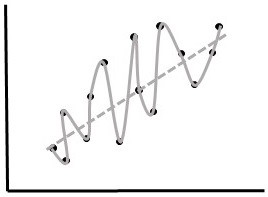
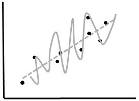
Comparison of performance of two algorithms (grey lines) on hypothetical training (A) and test (B) data (black points).
b: Test Data. Algorithm 1 (solid line) modeled the training data perfectly, but has very high error on the test data. Algorithm 2 had a higher error on the training data, but models the test data with a reasonably low error. Algorithm 1 is an example of overfitting. Algorithm 2 is a much better real-world predictor.
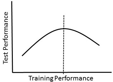
As algorithm performance on training data increases, performance on test data increases only to a certain point (dashed line). Increases in performance on training data beyond this point results in overfitting.
2) Favoring Complexity Over Simplicity. It is important for a problem to be addressed with just the right amount of complexity and this varies according to the nature of the problem and the data (e.g.
3) Including As Many Features As Possible. It can be difficult to know a priori which features are important predictors in a given problem, but including a large number of features in a model (i.e. a shotgun approach), especially features that are not relevant, can make a model a poor predictor
The second type of limitation results from not recognizing imperfections in data sets (
1) Class imbalance. This problem occurs when one or more classes are underrepresented compared to the others (
2) Too many categories. This problem is related to the Curse of Dimensionality and it occurs when a category has a high number of distinct values (i.e. high cardinality,
3) Missing data. Different types of learners and problems have different levels of tolerance for missing data during training, testing, and prediction (see discussion of ML techniques below). There are several methods for applying ML techniques to data with missing values (
4) Outliers. If the observations are real and not the result of human error, outliers can be an important source of insight. They only become a problem when they go unnoticed and models are applied to a data set as though outliers are not present. There are many methods for outlier detection that are recommended as a preprocessing step before ML (
Machine Learning Techniques
Tree-based Methods
Tree-based ML methods include decision trees, classification trees, and regression trees (
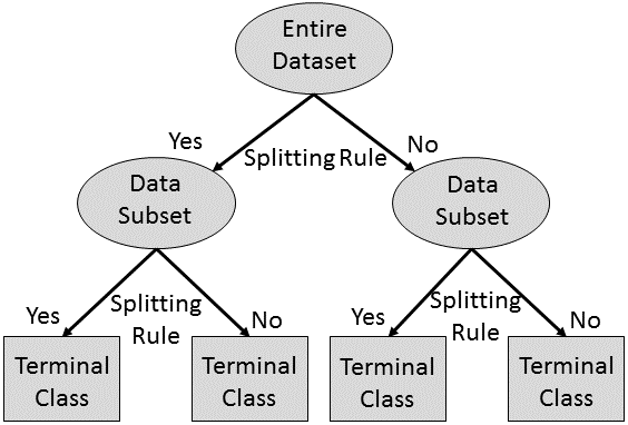
Decision and Classification Tree Schematic: Tree-based machine learning methods infer rules for splitting a data set into more homogeneous data sets until a specified number of terminal classes or maximum variance within the terminal classes is reached. The inferred splitting rules can give additional information about the system being studied.
Random Forest is a relatively new tree-based method that fits a user-selected number of trees to a data set and then combines the predictions from all trees (
Ensemble tree-based methods, especially Random Forest, have been demonstrated to outperform traditional statistical methods and other ML methods in earth science and ecology applications (
For a more detailed description of tree-based methods see
Artificial Neural Networks
An Artificial Neural Network (ANN) is a ML approach inspired by the way neurological systems process information (
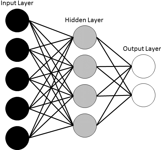
Artificial Neural Network Schematic: A neural network is made up of three layers (input, hidden, output). Each layer contains interconnected units (neurons). Each connection has an assigned connection weight. The number of hidden units and the connection weights are iteratively improved to minimize the error between the output and the target.
ANN can be a powerful modeling tool when the underlying relationships are unknown and the data are imprecise and noisy (
For a more detailed description of a multi-layer, feed-forward ANN with back propagation see section 4.1 in
Support Vector Machines
A Support Vector Machine (SVM) is a type of binary classifier. Data are represented as points in space and classes are divided by a straight line "margin". The SVM maximizes the margin by placing the largest possible distance between the margin and the instances on both sides (Fig.
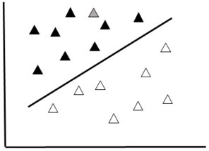
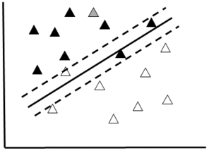
Support Vector Machine Schematic
b: If the data are noisy, and not easily separated, a “soft margin” (dotted lines) can be used to separate the two classes.
SVM is well suited for problems with many features compared to instances (Curse of Dimensionality) and is capable of avoiding problems with local minima (
For a more detailed description of SVMs see section 6 in
Genetic Algorithm
Genetic Algorithms (GA) are based on the process of evolution in natural systems in that a population of competing solutions evolves over time to converge on an optimal solution (
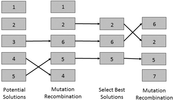
Genetic Algorithm Schematic: In this simplified schematic of a genetic algorithm, the five potential solutions, or “chromosomes”, undergo mutation and recombination. Then the best performing solutions are selected for another iteration of mutation and recombination. This cycle is repeated until an optimal solution is found.
An advantage of GA is the removal of the often arbitrary process of choosing a model to apply to the data (
For a more detailed discussion of GA see
Fuzzy Inference Systems
Fuzzy inference methods, such as Fuzzy Logic and Inductive Logic Programming, provide a practical approach to automating complex analysis and inference in a long workflow (
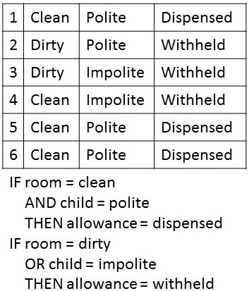
Fuzzy Inference Rule Set. This is a simplified example of an "if/then" rule set derived from data (in the table) using fuzzy inference. The inferred rules can be used to predict when an allowanced with be dispensed.
Fuzzy inference systems perform a rule induction task. The resulting rules can be easy to understand and interpret, as long as the rule sets are not too large, but overfitting can be a problem (
For more information about fuzzy inference systems and rule induction see
Bayesian Methods
Bayesian ML methods are based on Bayesian statistical inference, which started in the 18th century with the development of Bayes’ theorem (
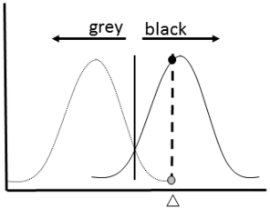
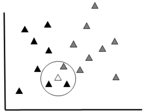
Bayesian Classifier Schematic: This diagram shows a simplified schematic of a Bayesian classifier working to assign a new datum (white triangle) to one of two classes (grey and black).
b: Data Plot: An object to be classified (white) can belong to one of two groups (grey or black). This method would classify the object within the group with the highest probability of being correct. In this example, the white item would be classified as a member of the black group because the probability is higher (Black = 8/17 * 2/8 and Grey = 9/17 *1/9)
A Bayesian classifier gives good results in most cases and requires fewer training data compared to other ML methods (
For a more detailed discussion of Bayesian Classifiers and Bayesian Networks see section 5.1 in
Using ML in Ecology and Earth Science
For many researchers, machine learning is a relatively new paradigm that has only recently become accessible with the development of modern computing. While the adoption of ML methods in earth science and ecology has been slow, there are several published studies using ML in these disciplines (e.g.,
Habitat Modeling and Species Distribution
Understanding the habitat requirements of a species is important for understanding its ecology and managing its conservation. Habitat modelers are interested in using multiple data sets to make predictions and classifications about habitat characteristics and where taxa are likely to be located or engaging in a specific behavior (e.g., nesting
Species Identification
Identifying taxa can require specialized knowledge only possessed by a very few and the data set requiring expert curation can be large (e.g., automated collection of images and sounds). Thus, the expert annotation step is a major bottleneck in biodiversity studies. In order to increase throughput, algorithms are trained on images, sounds, and other types of data labeled with taxon names. (For more information about automated taxon identification specifically, see
Remote Sensing
Satellite images and other data gathered from sensors at great elevation (e.g., LIDAR) are an excellent way to gather large amounts of data about Earth over broad spatial scales. In order to be useful, these data must go through some minimum level of processing (
Resource Management
Making decisions about conservation and resource management can be very difficult because there is often not enough data for certainty and the consequences of being wrong can be disastrous. ML methods can provide a means of increasing certainty and improving results, especially techniques that incorporate Bayesian probabilities. Several algorithms have been applied to water (
Forecasting
Discovery of deterministic chaos in meteorological models (
Environmental Protection and Safety
Just as ML can help resource managers make important decisions with or without adequate data coverage, environmental protection and safety decisions can be aided with ML methods when data are sparse. ML has been used to classify environmental samples into inferred quality classes in situations where direct analyses are too costly (
Climate Change Studies
One of the more pressing societal problems is the mitigation of and adaptation to climate change. Policy-makers require well-formed predictions in order to make decisions, but the complexity of the climate system, the interdisciplinary nature of the problem, and the data structures prevents the effective use of linear modeling techniques. ML is used to study important processes such as El Niño, the Quasi Biennial Oscillation, the Madden-Julian Oscillation, and monsoon modes (
Discussion
How can ML advance ecology and earth science?
The application of ML methods in ecology and earth science has already demonstrated the potential for increasing the quality and accelerating the pace of science. One of the more obvious ways ML does this is by coping with data gaps. The Earth is under-sampled, despite spending hundreds of millions of dollars on earth and environmental science (e.g.,
ML can accelerate the pace of science by quickly performing complex classification tasks normally performed by a human. A bottleneck in many ecology and earth science workflows are the manual steps performed by an expert, usually a classification task such as identifying a species. Expert annotation can be even more time consuming when the expert must search through a large volume of data, like a sensor stream, for a desired signal (
As discussed above, ML techniques can perform better than traditional statistical methods in some systems, but a direct comparison of performance between ML techniques and traditional statistical methods is difficult because there is no universal measure of performance and results can be very situation-specific (
Why don’t more people use ML?
Even though ML can outperform traditional statistics in some applications (
Another barrier to using ML techniques is the need for adequate amounts of training and test data within the desired range of prediction. This places an important constraint on the application of ML to problems that have appropriate, annotated data sets available. For example, the Google image recognition algorithm was developed using 1.2 million annotated images (
This combination of lack of formal education and important data restrictions can lead to naive applications of ML techniques, which can increase resistence to their adoption.
Finally, communication between the ML research community and natural science research community is poor (
Next Steps
How can the use of ML methods in ecology and earth science be encouraged? One barrier that has been partially lowered is the lack of tools and services to support the application of ML in these domains. Use of ML algorithms built with user infrastructure, such as GRASS-GIS (
Research scientists want to have a good understanding of the algorithms they use, which makes adoption of a new method a non-trivial investment. Reducing the cost of this investment for ML techniques is an important part of encouraging adoption. One way to do this is through a trusted collaborator who can simultaneously guide the research and transfer skills. These collaborators can be difficult to find, but many potential partners can be found in industry. A useful tool would be a publicly-available repository of annotated data sets to act as a sandbox for researchers wanting to learn and experiment with these methods, similar to Kaggle (https://www.kaggle.com/) but with natural science data. Random Forest is easier for a beginner to implement, gives easy to interpret results, and has high performance on ecology and earth science classification problems (
Finally, ML successes and impacts in ecology and earth science need to be more effectively communicated and the results from ML analyses need to be easily interpreted for decision-makers (
Funding agencies can facilitate this process by specifically soliciting new collaborative projects (research projects, workshops, hack-a-thons, conference sessions) that apply ML methods to ecology and earth science in innovative ways and initiatives to develop education materials for natural science students. Proper implementation of ML methods requires an understanding of the data science and the discipline that can best be achieved through interdisciplinary collaboration.
Conclusions
ML methods offer a diverse array of techniques, now accessible to individual researchers, that are well suited to the complex data sets coming from ecology and earth science. These methods have the potential to improve the quality of scientific research by providing more accurate models and accelerate progress in science by widening bottlenecks, filling data gaps, and enhancing understanding of how systems work. Application of these methods within the ecology and earth science domain needs to increase if society is to see the benefit. Adoption can be promoted through interdisciplinary collaboration, increased communication, increased formal and informal education, and financial support for ML research. Partnerships with companies interested in environmental issues can be an excellent source of knowledge transfer. A good introductory ML method is Random Forest, which is easy to implement and gives good results. However, ML methods have limitations and are not the answer to all problems. In some cases traditional statistical approaches are more appropriate (
There are many more types of ML methods and subtly different techniques than what has been discussed in this paper. Implementing ML effectively requires additional background knowledge. A very helpful series of lectures by Stanford Professors Trevor Hastie and Rob Tibshirani called “An Introduction to Statistical Learning with Applications in R” can be accessed online for free and gives a general introduction to traditional statistics and some ML methods. Kaggle (https://www.kaggle.com/) is an excellent source of independent, hands-on data science lessons. A suggested introductory text is "Machine Learning Methods in the Environmental Sciences", by William Hsieh (
Acknowledgements
The author would like to acknowledge NASA for financial support and the Boston Machine Learning Meetup Group for inspiration. This paper was greatly improved by comments from Ronny Peters (reviewer), Christopher W. Lloyd, Holly A. Bowers, Alan H. Fielding, and Joseph Gormley.
References
- Automated classification of bird and amphibian calls using machine learning: A comparison of methods.Ecological Informatics4(4):206‑214. https://doi.org/10.1016/j.ecoinf.2009.06.005
- Introduction to Machine Learning.The MIT Press,615pp.
- A comparison of supervised learning techniques in the classification of bat echolocation calls.Ecological Informatics5(6):465‑473. https://doi.org/10.1016/j.ecoinf.2010.08.001
- Introduction Neural networks in remote sensing.International Journal of Remote Sensing18(4):699‑709. https://doi.org/10.1080/014311697218700
- Does science advance one funeral at a time?National Bureau of Economic Research21788:1. https://doi.org/10.3386/w21788
- Automatic identification of algae: neural network analysis of flow cytometric data.J Plankton Res14(4):575‑589. https://doi.org/10.1093/plankt/14.4.575
- Stochastic models that predict trouts population densities or biomass on macrohabitat scale.Hydrobiologia337:1‑9.
- Bell J (1999) Tree-based methods. In: Fielding AH (Ed.) Machine Learning Methods for Ecological Applications.Springer US,New York,89-106pp.
- Support vector clustering.Journal of Machine Learning Research2:125‑137.
- Australian sea-floor survey data, with images and expert annotations.Scientific Data2:150057. https://doi.org/10.1038/sdata.2015.57
- Machine learning for bioclimatic modelling.Int J Adv Comput Sci Appl4(2):8.
- Pattern Recognition and Machine Learning.Springer-Verlag,New York,738pp. [ISBN978-0-387-31073-2]
- Predicting the conservation status of data-deficient species.Conservation Biology29(1):250‑259. https://doi.org/10.1111/cobi.12372
- Boddy L, Morris C (1999) Artificial neural networks for pattern recognition. In: Fielding AH (Ed.) Machine Learning Methods for Ecological Applications.Springer US,New York,37-88pp.
- Neural network analysis of flow cytometric data for 40 marine phytoplankton species.Cytometry15(4):283‑293. https://doi.org/10.1002/cyto.990150403
- Bagging predictors.Machine Learning24(2):123‑140. https://doi.org/10.1023/a:1018054314350
- Statistical modeling: The two cultures.Stat Sci16(3):199‑231.
- Random Forests.Machine Learning45(1):5‑32. https://doi.org/10.1023/a:1010933404324
- Classification and Regression Trees.Chapman Hall/CRC Press,368pp. [ISBN0412048418]
- Artificial neural network versus multiple linear regression: Predicting P/B ratios from empirical data.Marine Ecology Progress Series140:251‑256.
- Abundance, diversity, and structure of freshwater invertebrates and fish communities: An artificial neural network approach.New Zealand Journal of Marine and Freshwater Research35(1):135‑145. https://doi.org/10.1080/00288330.2001.9516983
- A simulated map of the potential natural forest vegetation of Switzerland.J Veg Sci4(4):499‑508. URL: http://www.jstor.org/stable/3236077
- Coastal typology: An integrative "neutral" technique for coastal zone characterization and analysis.Estuarine and Coastal Shelf Science77(2):197‑205. https://doi.org/10.1016/j.ecss.2007.09.021
- Specification of training sets and the number of hidden neurons for multilayer perceptrons.Neural Comput13(12):2673‑2680.
- Linear and nonlinear postprocessing of numerical forecasted surface temperature.Nonlinear Process Geophys10:373‑383.
- Intraseasonal variability associated with wet monsoons in southeast Arizona.Journal of Climate2002(15):2477‑2490. https://doi.org/10.1175/1520-0442(2002)0152.0.CO;2
- Chawla N (2005) Data mining for imbalanced datasets: An overview. In: Maimon O, Rokach L (Eds) The Data Mining and Knowledge Discovery Handbook.Springer,853-867pp. https://doi.org/10.1007/0-387-25465-X_40
- A fuzzy logic model with genetic algorithm for analyzing fish stock-recruitment relationships.Can. J. Fish. Aquat. Sci.57(9):1878‑1887. https://doi.org/10.1139/f00-141
- Automated bioacoustic identification of species.Ann Brazilian Acad Sci76(2):435‑440.
- Patternizing commuinities by using an artificial neural network.Ecological Modelling90:69‑78. https://doi.org/10.1016/0304-3800(95)00148-4
- Intelligent Strategies for Effective Quantitative Structure-Toxicity Relationship (QSTR) Screening.in proof1:1.
- Classifying individuals among infraspecific taxa using microsatellite data and neural networks.Comptes Rendus l’Académie des Sci Série III, Sci la vie319(12):1167‑1177.
- Do experts make mistakes? A comparison of human and machine identification of dinoflagellates.Marine Ecology Progress Series247:17‑25. https://doi.org/10.3354/meps247017
- Random forests for classification in ecology.Ecology88(11):2783‑2792. https://doi.org/10.1890/07-0539.1
- Ecological uses for genetic algorithms: predicting fish distributions in complex physical habitats.Can. J. Fish. Aquat. Sci.52(9):1893‑1908. https://doi.org/10.1139/f95-782
- Boosted trees for ecological modeling and prediction.Ecology81:243‑251. https://doi.org/10.1890/0012-9658(2007)88[243:BTFEMA]2.0.CO;2
- Classification and regression trees: A powerful yet simple technique for ecological data analysis.Ecology81(11):3178‑3192.
- Habitat suitability modelling for red deer (Cervus elaphus L.) in South-central Slovenia with classification trees.Ecol Modell138:321‑330. https://doi.org/10.1016/S0304-3800(00)00411-7
- Optimization of Artificial Neural Network (ANN) model design for prediction of macroinvertebrates in the Zwalm river basin (Flanders, Belgium).Ecological Modelling174:161‑173. https://doi.org/10.1016/j.ecolmodel.2004.01.003
- A test of a pattern recognition system for identification of spiders.Bull Entomol Res89:217‑224.
- A few useful things to know about machine learning.Communications of the ACM55(10):78‑87. https://doi.org/10.1145/2347736.2347755
- Modelling ecological niches with support vector machines.J Appl Ecology43(3):424‑432. https://doi.org/10.1111/j.1365-2664.2006.01141.x
- Clustering: A neural network approach.Neural Networks23(1):89‑107. https://doi.org/10.1016/j.neunet.2009.08.007
- Support vector machines regression for retrieval of leaf area index from multiangle imaging spectroradiometer.Remote Sensing of Environment107:348‑361. https://doi.org/10.1016/j.rse.2006.09.031
- A comparison of pixel-based and object-based image analysis with selected machine learning algorithms for the classification of agricultural landscapes using SPOT-5 HRG imagery.Remote Sensing of Environment118:259‑272. https://doi.org/10.1016/j.rse.2011.11.020
- Applications of symbolic machine learning to ecological modelling.Ecol Modell146:263‑273. https://doi.org/10.1016/S0304-3800(01)00312-X
- Džeroski S (2009) Machine learning applications in habitat suitability modeling. In: Haupt S, Pasini A, Marzban C (Eds) Artificial Intelligence Methods in the Environmental Sciences.Springer Netherlands,Amsterdam,397-412pp.
- Proceedings of the Ninth International Conference on Inductive Logic Programming.Springer,80-81pp.
- Expert systems: frames, rules or logic for species identification?Bioinformatics3(1):1‑7. https://doi.org/10.1093/bioinformatics/3.1.1
- Model-based stratifications for enhancing the detection of rare ecological events.Ecology86(5):1081‑1090. https://doi.org/10.1890/04-0608
- A working guide to boosted regression trees.Journal of Animal Ecology77(4):802‑813. https://doi.org/10.1111/j.1365-2656.2008.01390.x
- Novel methods improve prediction of species’ distributions from occurrence data.Ecography29(2):129‑151. https://doi.org/10.1111/j.2006.0906-7590.04596.x
- A Comparison of Outlier Detection Algorithms for Machine Learning.CiteSeerx2005:e. https://doi.org/10.1.1.61.5991
- Bird Species Recognition Using Support Vector Machines.EURASIP Journal on Advances in Signal Processing2007(1):038637. https://doi.org/10.1155/2007/38637
- Proceedings of CEC-2000, conference on evolutionary computation,1.La Jolla, USA.805-811pp.
- Machine Learning Methods for Ecological Applications.Springer US,New York,261pp.
- Fielding AH (1999) An introduction to machine learning methods. In: Fielding AH (Ed.) Machine Learning Methods for Ecological Applications.Springer US,New York,1-36pp.
- Cluster and Classification Techniques in the BioSciences.Cambridge University Press,Cambridge,260pp. [ISBN9780521618007]
- Simulating the distribution of plant communities in an alpine landscape.Coenoses5:37‑43.
- Proceedings of the XVII Congress ASPRS.570-573pp.
- Fletcher T (2016) Machine Learning for Financial Market Prediction.University College London,Department of Computer Science,207pp.
- ECCO version 4: an integrated framework for non-linear inverse modeling and global ocean state estimation.Geoscientific Model Development Discussions8(5):3653‑3743. https://doi.org/10.5194/gmdd-8-3653-2015
- Proceedings of the 3rd International Workshop on Distributed Statistical Computing.
- Fürnkranz J, Gamberger D, Lavrač N (2012) Rule Learning in a Nutshell. In: Fürnkranz J, Gamberger D, Lavrač N (Eds) Foundations of Rule Learning.Springer,19-55pp.
- Foundations of Rule Learning.Springer,334pp. https://doi.org/10.1007/978-3-540-75197-7
- Gamberger D, Sekusak S, Medven Z, Sabljic A (1996) Application of Artificial Intelligence in Biodegradation Modelling. In: Peijnenburg WGM, Damborský J (Eds) Biodegradability Prediction.Springer,41-50pp. https://doi.org/10.1007/978-94-011-5686-8_5
- Gantayat SS, Misra A, Panda BS (2014) A Study of Incomplete Data – A Review. In: Satapathy SC, Udgata SK, Biswal BN (Eds) Advances in Intelligent Systems and Computing.Springer,563pp. https://doi.org/10.1007/978-3-319-02931-3_45
- Predicting habitat suitability with machine learning models: The potential area of Pinus sylvestris L. in the Iberian Peninsula.Ecological Modelling197:383‑393. https://doi.org/10.1016/j.ecolmodel.2006.03.015
- Classes of Kernels for Machine Learning: A Statistics Perspective.Journal of Machine Learning Research2:299‑312.
- Modelling spatial dynamics of fish.Reviews in Fish Biology and Fisheries8(1):57‑91. https://doi.org/10.1023/a:1008864517488
- Random Forests for land cover classification.Pattern Recognition Letters27(4):294‑300. https://doi.org/10.1016/j.patrec.2005.08.011
- Genetic algorithms and machine learning.Machine Learning3:95‑99. https://doi.org/10.1023/a:1022602019183
- Evaluating and improving a semi-automated image analysis technique for identifying bivalve larvae.Limnol. Oceanogr.12(8):548‑562. https://doi.org/10.4319/lom.2014.12.548
- Energy availability and habitat heterogeneity predict global riverine fish diversity.Nature391(6665):382‑384. https://doi.org/10.1038/34899
- Predicting species distribution: offering more than simple habitat models.Ecology Letters8(9):993‑1009. https://doi.org/10.1111/j.1461-0248.2005.00792.x
- Predictive habitat distribution models in ecology.Ecol Modell135(2):147‑186. https://doi.org/10.1016/S0304-3800(00)00354-9
- Predicting species distributions for conservation decisions.Ecology Letters16(12):1424‑1435. https://doi.org/10.1111/ele.12189
- Support vector machines for predicting distribution of Sudden Oak Death in California.Ecological Modelling182(1):75‑90. https://doi.org/10.1016/j.ecolmodel.2004.07.012
- Modeling Biological Systems: Principles and Applications.Springer US,New York,475pp. https://doi.org/10.1007/b106568
- Neural Network Design.Martin Hagan,1012pp.
- Investigation of the random forest framework for classification of hyperspectral data.IEEE Trans. Geosci. Remote Sensing43(3):492‑501. https://doi.org/10.1109/tgrs.2004.842481
- Practical Genetic Algorithms.John Wiley & Sons Inc.,253pp. https://doi.org/10.1002/0471671746
- Haupt S (2009) Environmental optimization: Applications of genetic algorithms. In: Haupt S, Pasini A, Marzban C (Eds) Artificial Intelligence Methods in the Environmental Sciences.Springer Netherlands,Amsterdam,379-396pp.
- Haupt S, Allen C, Young G (2009) Addressing air quality problems with genetic algorithms: A detailed analysis of source characterization. In: Haupt S, Pasini A, Marzban C (Eds) Artificial Intelligence Methods in the Environmental Sciences.Springer Netherlands,Amsterdam,269-296pp.
- Artificial Intelligence Methods in the Environmental Sciences.Springer Netherlands,Amsterdam,424pp. https://doi.org/10.1007/978-1-4020-9119-3
- The Problem of Overfitting.Journal of Chemical Information and Computer Sciences44(1):1‑12. https://doi.org/10.1021/ci0342472
- Australia-wide predictions of soil properties using decision trees.Geoderma124:383‑398. https://doi.org/10.1016/j.geoderma.2004.06.007
- Adaptation in Natural and Artificial Systems: An Introductory Analysis with Applications to Biology, Control, and Artificial Intelligence.MIT Press,Cambridge,211pp.
- Machine Learning Methods in the Environmental Sciences.Cambridge University Press,Cambridge,349pp. [ISBN978-0-521-79192-2]
- An adaptive nonlinear MOS scheme for precipitation forecasts using neural networks.Weather Forecast18:303‑310. https://doi.org/10.1175/1520-0434(2003)0182.0.CO;2
- A machine-learning approach to automated knowledge-base building for remote sensing image analysis with GIS data.Photogramm Eng Remote Sens63(10):1185‑1194.
- Iverson L, Prasad A, Liaw A (2004) New machine learning tools for predictive vegetation mapping after climate change: Bagging and random forest perform better than regression tree analysis. In: Smithers R (Ed.) Landscape Ecology of Trees and Forests, Proceedings of the Twelfth Annual IALE(UK) Conference.International Association for Landscape Ecology,317-320pp.
- Data clustering: 50 years beyond K-means.Pattern Recognition Letters31(8):651‑666. https://doi.org/10.1016/j.patrec.2009.09.011
- An Introduction to Statistical Learning.Springer,426pp.
- The class imbalance problem: A systematic study.Intelligent Data Analysis6(5):429‑449.
- Jeffers J (1999) Genetic Algorithms I. In: Fielding AH (Ed.) Machine Learning Methods for Ecological Applications.Springer Netherlands,Amsterdam,107-122pp.
- Human vs. machine: identification of bat species from their echolocation calls by humans and by artificial neural networks.Can. J. Zool.86(5):371‑377. https://doi.org/10.1139/z08-009
- Missing data imputation using statistical and machine learning methods in a real breast cancer problem.Artificial Intelligence in Medicine50(2):105‑115. https://doi.org/10.1016/j.artmed.2010.05.002
- Analysing Extinction Risk in Parrots using Decision Trees.Biodivers Conserv15(6):1993‑2007. https://doi.org/10.1007/s10531-005-4316-1
- Application of machine learning techniques to the analysis of soil ecological data bases: Relationships between habitat features and Collembolan community characteristics.Soil Biol Biochem32(2):197‑209. https://doi.org/10.1016/S0038-0717(99)00147-9
- Classification in conservation biology: A comparison of five machine-learning methods.Ecological Informatics5(6):441‑450. https://doi.org/10.1016/j.ecoinf.2010.06.003
- Ensemble extraction for classification and detection of bird species.Ecological Informatics5(3):153‑166. https://doi.org/10.1016/j.ecoinf.2010.02.003
- Feedforward backpropagation neural networks in prediction of farmer risk preference.Am J Agric Econ78(2):400‑415. URL: http://www.jstor.org/stable/1243712
- Convergence of a Generalized SMO Algorithm for SVM Classifier Design.Machine Learning46:351‑360. https://doi.org/10.1023/a:1012431217818
- Keogh E, Mueen A (2011) Curse of Dimensionality. In: Sammut C, Webb G (Eds) Encyclopedia of Machine Learning.Springer,257-258pp. https://doi.org/10.1007/978-0-387-30164-8_192
- New approaches to modelling fish–habitat relationships.Ecological Modelling221(3):503‑511. https://doi.org/10.1016/j.ecolmodel.2009.11.008
- Predictive mapping of reef fish species richness, diversity and biomass in Zanzibar using IKONOS imagery and machine-learning techniques.Remote Sensing of Environment114(6):1230‑1241. https://doi.org/10.1016/j.rse.2010.01.007
- Identifying brown bear habitat by a combined GIS and machine learning method.Ecol Modell135:291‑300. https://doi.org/10.1016/S0304-3800(00)00384-7
- Self-Organization and Associative Memory.Springer Series in Information Sciences,312pp. https://doi.org/10.1007/978-3-642-88163-3
- Information complexity of neural networks.Neural Netw13(3):365‑375.
- Supervised Machine Learning: A Review of Classification Techniques.Informatica31:249‑268.
- Machine learning: a review of classification and combining techniques.Artificial Intelligence Review26(3):159‑190. https://doi.org/10.1007/s10462-007-9052-3
- Genetic Programming: On the Programming of Computers by Means of Natural Selection.MIT Press,Cambridge,836pp.
- Krasnopolsky V (2009) Neural network applications to solve forward and inverse problems in atmospheric and oceanic satellite remote sensing. In: Haupt S, Pasini A, Marzban C (Eds) Artificial Intelligence Methods in the Environmental Sciences.Springer Netherlands,Amsterdam,191-206pp.
- Lakshmanan V (2009) Automated analysis of spatial grids. In: Haupt S, Pasini A, Marzban C (Eds) Artificial Intelligence Methods in the Environmental Sciences.2009.Springer Netherlands,Amsterdam,329-346pp.
- Memoir on the Probability of the Causes of Events.Statistical Science1(3):364‑378. https://doi.org/10.1214/ss/1177013621
- Predicting climate-induced range shifts: Model differences and model reliability.Glob Chang Biol12(8):1568‑1584.
- Classification of breeding bird communities along an urbanization gradient using an unsupervised artificial neural network.Ecological Modelling203:62‑71. https://doi.org/10.1016/j.ecolmodel.2006.04.033
- Lees B (1996) Sampling strategies for machine learning using GIS. In: Goodchild M, Steyaert L, Parks B, Johnston C, Maidment D, Crane M, Glendinning S (Eds) GIS and Environmental Modeling: Progress and Issues.GIS World Inc.,Fort Collins,39-42pp. [ISBN978-0-470-23677-2].
- Decision-tree and rule-induction approach to integration of remotely sensed and GIS data in mapping vegetation in disturbed or hilly environments.Environmental Management15(6):823‑831. https://doi.org/10.1007/bf02394820
- Artificial neural networks as a tool in ecological modelling, an introduction.Ecological Modelling120:65‑73. https://doi.org/10.1016/S0304-3800(99)00092-7
- Artificial Neuronal Networks: Application to Ecology and Evolution.Springer Verlag,Berlin,262pp. https://doi.org/10.1007/978-3-642-57030-8
- Role of some environmental variables in trout abundance models using neural networks.Aquat. Living Resour.9(1):23‑29. https://doi.org/10.1051/alr:1996004
- Application of neural networks to modelling non linear relationships in ecology.Ecol Modell90:39‑52. https://doi.org/10.1016/0304-3800(95)00142-5
- Classifying soil-structure using neural networks.Ecol Modell92:101‑108.
- Application of machine learning methods to spatial interpolation of environmental variables.Environmental Modelling & Software26(12):1647‑1659. https://doi.org/10.1016/j.envsoft.2011.07.004
- A comparison of prediction accuracy, complexity, and training time of thirty three old and new classification algorithms.Machine Learning40(3):203‑228. https://doi.org/10.1023/a:1007608224229
- Fifty Years of Classification and Regression Trees.International Statistical Review82(3):329‑348. https://doi.org/10.1111/insr.12016
- Comparing machine learning classifiers in potential distribution modelling.Expert Systems with Applications38(5):5268‑5275. https://doi.org/10.1016/j.eswa.2010.10.031
- Deterministic non-periodic flow.J Atmos Sci20:130‑141.
- Automated Taxon Identification in Systematics: Theory, Approaches and Applications.CRC Press,368pp. [ISBN9780849382055]
- Neural networks for the prediction and forecasting of water resource variables: A review of modelling issues and applications.Environ Model Softw15(1):101‑124. https://doi.org/10.1016/S1364-8152(99)00007-9
- Alternative methods for predicting species distribution: an illustration with Himalayan river birds.J Appl Ecology36(5):734‑747. https://doi.org/10.1046/j.1365-2664.1999.00440.x
- A neural network for post-processing model output: ARPS.Mon Weather Rev131:1103‑1111.
- The use of artificial neural networks to predict the presence of small-bodied fish in a river.Freshwater Biology38(2):237‑246. https://doi.org/10.1046/j.1365-2427.1997.00209.x
- Variants of genetic programming for species distribution modelling - fitness sharing, partial functions, population evaluation.Ecol Modell146:231‑241. https://doi.org/10.1016/S0304-3800(01)00309-X
- Application of neural networks to prediction of fish diversity and salmonid production in the Lake Ontario basin.Trans Am Fish Soc134(1):28‑43.
- What do we gain from simplicity versus complexity in species distribution models?Ecography37(12):1267‑1281. https://doi.org/10.1111/ecog.00845
- Predicting species distributions: a critical comparison of the most common statistical models using artificial species.Journal of Biogeography34(8):1455‑1469. https://doi.org/10.1111/j.1365-2699.2007.01720.x
- A preprocessing scheme for high-cardinality categorical attributes in classification and prediction problems.ACM SIGKDD Explorations Newsletter3(1):27. https://doi.org/10.1145/507533.507538
- Modelling distribution of four vegetation alliances using generalized linear models and classification trees with spatial dependence.Ecol Modell157:227‑247. https://doi.org/10.1016/S0304-3800(02)00196-5
- An Introduction to Genetic Algorithms.MIT Press,Cambridge,221pp.
- Including high-cardinality attributes in predictive models: A case study in churn prediction in the energy sector.Decision Support Systems72:72‑81. https://doi.org/10.1016/j.dss.2015.02.007
- Support vector machines with applications.Statistical Science21(3):322‑336.
- Support vector machines in remote sensing: A review.ISPRS Journal of Photogrammetry and Remote Sensing66(3):247‑259. https://doi.org/10.1016/j.isprsjprs.2010.11.001
- Inverse entailment and progol.New Generation Computing13:245‑286. https://doi.org/10.1007/bf03037227
- Genetic algorithms for calibrating water quality models.J Environ Eng124(3):202‑211. https://doi.org/10.1061/(ASCE)0733-9372(1998)124:3(202)
- Genetic programming for analysis and real-time prediction of coastal algal blooms.Ecological Modelling189:363‑376. https://doi.org/10.1016/j.ecolmodel.2005.03.018
- Machine Learning Methods Without Tears: A Primer for Ecologists.The Quarterly Review of Biology83(2):171‑193. https://doi.org/10.1086/587826
- Machine learning techniques for anomaly detection: An overview.International Journal of Computer Applications79(2):33‑41.
- Methodological issues in building, training, and testing artificial neural networks in ecological applications.Ecological Modelling195:83‑93. https://doi.org/10.1016/j.ecolmodel.2005.11.012
- Random forest classifier for remote sensing classification.International Journal of Remote Sensing26(1):217‑222. https://doi.org/10.1080/01431160412331269698
- Biologically-inspired machine learning implemented to ecological informatics.Ecological Modelling203:1‑7. https://doi.org/10.1016/j.ecolmodel.2006.05.039
- Acoustic identification of twelve species of echoloating bat by discriminant function analysis and artificial neural networks.J Exp Biol203:2641‑2656.
- Pasini A (2009) Neural network modeling in climate change studies. In: Haupt S, Pasini A, Marzban C (Eds) Artificial Intelligence Methods in the Environmental Sciences.Springer Netherlands,Amsterdam,235-254pp.
- Random forests as a tool for ecohydrological distribution modelling.Ecological Modelling207:304‑318. https://doi.org/10.1016/j.ecolmodel.2007.05.011
- Future projections for Mexican faunas under global climate change scenarios.Nature416(6881):626‑629. https://doi.org/10.1038/416626a
- Generalization of back-propagation to recurrent neural networks.Phys. Rev. Lett.59(19):2229‑2232. https://doi.org/10.1103/physrevlett.59.2229
- Support vector machines to map rare and endangered native plants in Pacific islands forests.Ecological Informatics9:37‑46. https://doi.org/10.1016/j.ecoinf.2012.03.003
- Manifestation of an advanced fuzzy logic model coupled with Geo-information techniques to landslide susceptibility mapping and their comparison with logistic regression modelling.Environmental and Ecological Statistics18(3):471‑493. https://doi.org/10.1007/s10651-010-0147-7
- Newer Classification and Regression Tree Techniques: Bagging and Random Forests for Ecological Prediction.Ecosystems9(2):181‑199. https://doi.org/10.1007/s10021-005-0054-1
- Induction of logic programs: FOIL and related systems.New Generation Computing13:287‑312. https://doi.org/10.1007/bf03037228
- A statistical assessment of population trends for data deficient Mexican amphibians.PeerJ2:e703. https://doi.org/10.7717/peerj.703
- Gaussian Processes for Machine Learning.MIT Press,Cambridge,248pp. [ISBN026218253X]
- Individuality in the groans of fallow deer (Dama dama) bucks.J Zoology245(1):79‑84. https://doi.org/10.1111/j.1469-7998.1998.tb00074.x
- ANNA - artificial neural network model for predicting species abundance and succession of blue-green algae.Hydrobiologia349:47‑57.
- Applications of machine learning to ecological modelling.Ecol Modell146:303‑310. https://doi.org/10.1016/S0304-3800(01)00316-7
- Proceedings of the 5th International Symposium WATERMATEX’2000 on Systems Analysis and Computing in Water Quality Management.
- Comparative application of artificial neural networks and genetic algorithms for multivariate time-series modelling of algal blooms in freshwater lakes.J Hydroinformatics4(2):125‑133.
- Genetic Algorithms - Principles and Perspectives.Springer,332pp. https://doi.org/10.1007/b101880
- The relationships of seabird assemblages to physical habitat features in Pacific equatorial waters during spring 1984–1991.ICES Journal of Marine Science54(4):593‑599. https://doi.org/10.1006/jmsc.1997.0244
- Mapping land-cover modifications over large areas: A comparison of machine learning algorithms.Remote Sens Environ112(5):2272‑2283. https://doi.org/10.1016/j.rse.2007.10.004
- Classification success of six machine learning algorithms in radar ornithology.Ibis158(1):28‑42. https://doi.org/10.1111/ibi.12333
- Ruck B, Walley W, Hawkes H (1993) Biological classification of river water quality using neural networks. In: Rzevski G, Pastor J, Adey R (Eds) Applications of Artificial Intelligence in Engineering VIII.Elsevier Applied Science,361-372pp.
- Rumelhart D, Hinton G, Williams R (1986) Learning internal representations by error propagation. In: Rumelhart D, McClelland J, Group P (Eds) Parallel Distributed Processing.MIT Press,Cambridge,318-362pp.
- Handling Missing Values when Applying Classification Models.Journal of Machine Learning Research8:1625‑1657.
- Biodiversity Conservation Planning Tools: Present Status and Challenges for the Future.Annual Review of Environment and Resources31(1):123‑159. https://doi.org/10.1146/annurev.energy.31.042606.085844
- Sastry K, Goldberg D, Kendall G (2013) Genetic Algorithms. Search Methodologies.Springer,93-117pp. https://doi.org/10.1007/978-1-4614-6940-7_4
- Artificial neural networks as empirical models for estimating phytoplankton production.Marine Ecology Progress Series139:289‑299.
- Developing an empirical model of phytoplankton primary production: a neural network case study.Ecological Modelling120:213‑223.
- Neural networks in agroecological modelling - stylish application or helpful tool?Computers and Electronics in Agriculture29(1):73‑97. https://doi.org/10.1016/S0168-1699(00)00137-X
- Neural Network Models of the Greenhouse Climate.Journal of Agricultural Engineering Research59(3):203‑216. https://doi.org/10.1006/jaer.1994.1078
- An evaluation of methods for modelling species distributions.Journal of Biogeography31(10):1555‑1568. https://doi.org/10.1111/j.1365-2699.2004.01076.x
- Modeling Ocean Circulation.Science269:1379‑1380.
- Neural Networks, 2001. Proceedings. IJCNN '01. International Joint Conference on.4.IJCNN'01.IEEE,2673-2678pp. https://doi.org/10.1109/ijcnn.2001.938792
- Species identification using wideband backscatter with neural network and discriminant analysis.ICES J Mar Sci.53:189‑195.
- Algorithms That Learn with Less Data Could Expand AI’s Power.MIT Technology Review601551:e. URL: https://www.technologyreview.com/s/601551/algorithms-that-learn-with-less-data-could-expand-ais-power/
- Biometry.W.H. Freeman,937pp. [ISBN0716786044]
- Automated taxonomic classification of phytoplankton sampled with imaging in flow cytometry.Limnol Oceanogr Methods5(6):204‑216. https://doi.org/10.4319/lom.2007.5.204
- Environmental impact prediction using neural network modelling. An example in wildlife damage.J Appl Ecology36(2):317‑326. https://doi.org/10.1046/j.1365-2664.1999.00400.x
- Srinivasan A, King R, Muggleton S, Sternberg M (1997) Carcinogenesis prediction using inductive logic programming. In: Lavrač N, Keravnou E, Zupan B (Eds) Intelligent Data Analysis in Medicine and Pharmacology.Springer US,New York,243-260pp.
- Stockwell D (1999) Genetic Algorithms II. In: Fielding AH (Ed.) Machine Learning Methods for Ecological Applications.Springer US,New York,123-144pp.
- Induction of sets of rules from animal distribution data: A robust and informative method of analysis.Math Comput Simul33:385‑390. https://doi.org/10.1016/0378-4754(92)90126-2
- The GARP modelling system: problems and solutions to automated spatial prediction.International Journal of Geographical Information Science13(2):143‑158. https://doi.org/10.1080/136588199241391
- The need for evidence-based conservation.Trends in Ecology & Evolution19(6):305‑308. https://doi.org/10.1016/j.tree.2004.03.018
- Predicting grassland community changes with an artificial neural network model. Ecol Modell.Ecological Modelling84:91‑97. https://doi.org/10.1016/0304-3800(94)00131-6
- The use of genetic algorithms and Bayesian classification to model species distributions.Ecological Modelling192:410‑424. https://doi.org/10.1016/j.ecolmodel.2005.07.009
- Data issues in the life sciences.ZooKeys150:15‑51. https://doi.org/10.3897/zookeys.150.1766
- BIOMOD - optimizing predictions of species distributions and projecting potential future shifts under global change.Global Change Biol9(10):1353‑1362. https://doi.org/10.1046/j.1365-2486.2003.00666.x
- Fuzzy classification of microbial biomass and enzyme activities in grassland soils.Soil Biology and Biochemistry39(7):1799‑1808. https://doi.org/10.1016/j.soilbio.2007.02.010
- Predicting occurrences and impacts of smallmouth bass introductions in north temperate lakes.Ecological Applications14(1):132‑148. https://doi.org/10.1890/02-5036
- Classification trees: An alternative non-parametric approach for predicting species distributions.Journal of Vegetation Science11(5):679‑694. https://doi.org/10.2307/3236575
- Proceedings of the International Joint Conference on Artificial Intelligence.IJCA1999.
- Wagstaff K (2012) Machine learning that matters. In: Langford J, Pineau J (Eds) Proceedings of the 29th International Conferene on Machine Learning.California Institute of Technology,298-303pp.
- Walley W, Džeroski S (1996) Biological monitoring: A comparison between Bayesian, neural and machine learning methods of water quality classification. In: Denzer R, Schimak G, Russell D (Eds) Environmental Software Systems: Proceedings of the International Symposium on Environmental Software Systems.Springer US,New York,229-240pp. https://doi.org/10.1007/978-0-387-34951-0_20
- Walley W, Hawkes H, Boyd M (1992) Application of Bayesian inference to river water quality surveillance. In: Grierson D, Rzevski G, Adey R (Eds) Applications of Artificial Intelligence in Engineering VII.Elsevier,1030-1047pp.
- Walley W, Martin R, O'Connor M (2000) Self-organising maps for the classification and diagnosis of river quality from biological and environmental data. In: Denzer R, Swayne D, Purvis M, Schimak G (Eds) Environmental Software Systems: Environmental Information and Decision Support.Springer US,New York,27-41pp.
- Fuzzy Logic.Springer,459pp. https://doi.org/10.1007/978-3-540-71258-9
- Naive Bayesian Classifier for Rapid Assignment of rRNA Sequences into the New Bacterial Taxonomy.Applied and Environmental Microbiology73(16):5261‑5267. https://doi.org/10.1128/aem.00062-07
- Biodiversity's Big Wet Secret: The Global Distribution of Marine Biological Records Reveals Chronic Under-Exploration of the Deep Pelagic Ocean.PLoS ONE5(8):e10223. https://doi.org/10.1371/journal.pone.0010223
- Wieland R (2008) Fuzzy models. In: Jørgensen S, Fath B (Eds) Encyclopedia of Ecology.Elsevier,Amsterdam,1717-1726pp.
- Adaptive fuzzy modeling versus artificial neural networks.Environmental Modelling & Software23(2):215‑224. https://doi.org/10.1016/j.envsoft.2007.06.004
- Niche Modeling Perspective on Geographic Range Predictions in the Marine Environment Using a Machine-learning Algorithm.Oceanography16(3):120‑127. https://doi.org/10.5670/oceanog.2003.42
- Williams J, Kessinger C, Abernathy J, Ellis S (2009) Fuzzy logic applications. In: Haupt S, Pasini A, Marzban C (Eds) Artificial Intelligence Methods in the Environmental Sciences.Springer Netherlands,Amsterdam,347-378pp.
- Modelling global insect pest species assemblages to determine risk of invasion.Journal of Applied Ecology43(5):858‑867. https://doi.org/10.1111/j.1365-2664.2006.01202.x
- Neural networks forecasts of the tropical Pacific sea surface temperatures.Neural Networks19:145‑154.
- Combinations of Evolutionary Computation and Neural Networks, 2000 IEEE Symposium on.San Antonio, Texas, USA.IEEE,168-175pp. https://doi.org/10.1109/ecnn.2000.886232
- Young G (2009) Implementing a neural network emulation of a satellite retrieval algorithm. In: Haupt S, Pasini A, Marzban C (Eds) Artificial Intelligence Methods in the Environmental Sciences.Springer Netherlands,Amsterdam,207-216pp.
- Bayesian Learning with Gaussian Processes for Supervised Classification of Hyperspectral Data.Photogrammetric Engineering & Remote Sensing74(10):1223‑1234. https://doi.org/10.14358/pers.74.10.1223
- Characterizing forest canopy structure with lidar composite metrics and machine learning.Remote Sensing of Environment115(8):1978‑1996. https://doi.org/10.1016/j.rse.2011.04.001