|
One Ecosystem :
Research Article
|
|
Corresponding author: Erik E Stange (Erik.Stange@nina.no)
Academic editor: Stoyan Nedkov
Received: 06 Jun 2017 | Accepted: 01 Nov 2017 | Published: 23 Nov 2017
© 2017 Erik Stange, Grazia Zulian, Graciela Rusch, David Barton, Megan Nowell
This is an open access article distributed under the terms of the Creative Commons Attribution License (CC BY 4.0), which permits unrestricted use, distribution, and reproduction in any medium, provided the original author and source are credited.
Citation:
Stange EE, Zulian G, Rusch GM, Barton D, Nowell M (2017) Ecosystem services mapping for municipal policy: ESTIMAP and zoning for urban beekeeping. One Ecosystem 2: e14014. https://doi.org/10.3897/oneeco.2.e14014
|
|
Abstract
Pollinating insects are an integral part of cities’ natural capital and perform an important ecosystem function with a high degree of relevance to many cultural ecosystem services. Consequently, pollinators serve as a useful proxy for assessing urban biodiversity. Beekeeping has recently emerged as a popular activity in many urban areas and a good deal of the motivation for urban beekeeping for many stems from the cultural and non-consumptive aspects of beekeeping. Yet the recent increases in domestic honeybee densities in urban landscapes has raised concern regarding the potential threat that honeybees might pose to local populations of threatened bumblebee and solitary bee species. This issue constitutes a trade-off between the cultural ecosystem services associated with urban beekeeping and the regulation and maintenance ecosystem services of maintaining nursery populations of rare and threatened species. Municipal authorities in Oslo, Norway have proposed establishing eight “precautionary zones”, within which placement of honeybee hives could be more strictly regulated. We propose a mapping and assessment approach for informing zoning decisions regarding urban honeybees, utilising a model of an urban landscape’s biophysical capacity to support pollinating insects (ESTIMAP). Together with an additional model describing the approximate distrubtion of honeybees in Oslo, we identify areas in the city where domestic honeybees may be more likely to exhaust floral resources. This case also tests the policy relevance of ecosystem service mapping tools beyond awareness raising, with broader general lessons for ecosystem mapping and assessment .
Keywords
Ecosystem services, Pollination, Honeybees, Wild bees, Urban, Mapping, Trade-offs
Introduction
Animal-mediated pollination is both an integral ecosystem process and a key ecosystem service (ES). With an estimated 87% of all flowering plant species dependent on insect pollinators for sexual reproduction (
The benefits humans derive from insect pollinators extend well beyond food production. Due to the ubiquitous role of insect pollination in sustaining wild plant populations, pollinators are also integral elements in many regulating and cultural ecosystem services . Either directly or indirectly, pollinators contribute to an improved quality of life for many people either through heritage, aesthetics or identity (
Few human activities integrate the elements of provisioning, regulating/maintenance and cultural ecosystem services as closely as beekeeping (or apiculture). As a primordial human domestication of nature (
Over half of world’s population and nearly three-quarters of Europe’s population lives in cities (
Public anxiety over the global status of bee populations is another motivating factor driving the recent increase in urban beekeeping’s popularity (
Wild bees are often more abundant than honeybees in urban areas (
Oslo municipality is home to Norway’s capital city. It is also the municipality with the country’s highest biodiversity, with the largest number of recorded observations of the country’s rare and red-listed species (
Seven of the proposed precautionary zones fall entirely within terrestrial portions of the Oslo municipality, with sizes ranging from 4 to 12 km2. The largest of the eight precautionary zones extends over nearly 60 km2, covering both the municipality’s entire coastline along the Oslo fjord and the many islands located within the municipality’s borders. Of the registered beehives located in Oslo in 2016, nearly half fell within these proposed zones. Oslo’s Urban Environmental Agency has presented these precautionary zones primarily as a tool for evaluating future applications for beehive permits and has not expressed the intention of demanding the removal of hives that presently fall within precautionary zones. Yet the overlap between the zones and the present location of so many beehives presents a potential for conflict, and both the agency and Oslo’s beekeeping community are interested in finding ways to objectively evaluate the appropriateness and necessity of this proposed zoning policy.
The situation in Oslo represents an interesting and illustrative example of a trade-off between biodiversity protection and a cultural ecosystem service. In this paper, we propose a mapping and assessment approach that can help inform zoning decisions regarding urban honeybees, utilising a model of an urban landscape’s biophysical capacity to support pollinating insects. As this model describes the spatial distribution of an important indicator of the broader urban biodiversity, the model also constitutes a non-monetary valuation approach (
Material and methods
2.1 Study area
Oslo is located in the northern innermost portion of the Oslo Fjord in Eastern Norway (59′55N, 10′45E). The city itself lies in a south-facing valley, with a local climate characterised by mild winters (average January temperature = -3°C), warm summers (average July temperature = 18°C) and a short but intense growing season (177 frost-free days · yr-1). The terrain slopes gently upwards from sea to the forested hills around the city (300 - 700 m a.s.l.). The Oslo municipality’s total area (454 km2) is home to 670 000 residents, which is a 20% increase since 2007 (
2.2 Modelling pollinator habitat suitability
We used a modified version of the ESTIMAP pollination model (
To model pollinator habitat suitability for a single urban setting, we used spatial data provided by Oslo municipality that defined polygons according to 33 land cover categories—including 14 different forest types (Table 1). We grouped the municipal classifications of forest types into six broader categories according to expert assessments of the forest attributes that pertain to the life histories of pollinating insects. We then differentiated between forest core and forest edge, defining forest edge as a 20 m wide band where forest polygons bordered non-forest land cover. We conferred with experts familiar with local pollinating insect taxa and used an iterative process to arrive at consensus values for land cover that express categories’ relative habitat suitability for the representative pollinating bee species occurring in Oslo. Land cover categories that are incapable of providing either floral resources or nesting sites (e.g. water surfaces or densely built areas) were valued at or near zero. Land cover categories that represent the best possible habitat within the study area were valued at 1. Based on the experts’ contention that nesting site availability was far less likely to limit populations of pollinating insects in Oslo than floral availability, we chose to simplify the ESTIMAP model for Oslo by using a combined habitat suitability score. Habitat suitability values also attempted to capture variation in the temporal availability of floral resources, such that only land cover categories expected to offer the most continuous availability of floral resources received full habitat suitability value (1).
We first used the ESTIMAP pollination spatial model for Oslo to calculate a habitat suitability score for 25 m raster cells. However, our preliminary validation analyses from insect sampling (described below) indicated that the spatial data provided by the municipality failed to capture the large degree of heterogeneity we observed in vegetation cover within many of the land cover categories. We therefore applied imagery from the Sentinel 2 satellite (at 10 m resolution) to improve the detail of the information in the land cover classes from the municipal land cover data. Sentinel 2 data included 13 spectral bands, plus Normalised Difference Vegetation Index (NDVI). We used a Random Forest classifier in R Studio (
|
Land cover category (from municipal data) |
Pixel habitat suitability score based on Sentinel 2 satellite land cover classification |
||||
|
Agricultural |
Low vegetation |
Tree |
Built |
Water |
|
|
core FNF (forest with no floral resources) |
0.1 |
0.4 |
0.1 |
0.1 |
0.05 |
|
core CO (conifer forest) |
0.2 |
0.6 |
0.3 |
0.1 |
0.05 |
|
core OF (other forest) |
0.3 |
0.5 |
0.4 |
0.1 |
0.05 |
|
core MFL (mixed forest low) |
0.4 |
0.6 |
0.5 |
0.1 |
0.05 |
|
core MFH (mixed forest high) |
0.3 |
0.8 |
0.6 |
0.1 |
0.05 |
|
core BLF (broad leaf forest) |
0.3 |
0.7 |
0.6 |
0.1 |
0.05 |
|
core FYF (forest with floral resources) |
0.4 |
0.7 |
0.7 |
0.1 |
0.05 |
|
edge FNF (forest with no floral resources) |
0.5 |
0.4 |
0.3 |
0.1 |
0.05 |
|
edge CO (conifer forest) |
0.6 |
0.9 |
0.8 |
0.2 |
0.05 |
|
edge OF (other forest) |
0.5 |
0.7 |
0.6 |
0.2 |
0.05 |
|
edge MFL (mixed forest low) |
0.6 |
1 |
0.9 |
0.2 |
0.05 |
|
edge MFH (mixed forest high) |
0.6 |
1 |
0.9 |
0.2 |
0.05 |
|
edge BLF (broad leaf forest) |
0.7 |
1 |
1 |
0.2 |
0.05 |
|
edge FYF (forest with floral resources) |
0.7 |
1 |
1 |
0.2 |
0.05 |
|
agricultural land |
0.3 |
0.6 |
0.6 |
0.1 |
0.05 |
|
medium built areas |
0.7 |
0.7 |
0.6 |
0.1 |
0.05 |
|
densely built areas |
0.35 |
0.45 |
0.25 |
0.05 |
0.05 |
|
mines |
0.35 |
0.55 |
0.35 |
0.05 |
0.05 |
|
graveyard |
0.5 |
0.9 |
0.7 |
0.1 |
0.05 |
|
industrial |
0.4 |
0.6 |
0.4 |
0.05 |
0.05 |
|
Transportation-infrastructures |
0.5 |
0.8 |
0.5 |
0.1 |
0.05 |
|
Sports-stadiums |
0.1 |
0.1 |
0.4 |
0.1 |
0.05 |
|
alpine ski area |
0.4 |
0.5 |
0 |
0.1 |
0.05 |
|
parks |
0.5 |
0.6 |
0.8 |
0.1 |
0.05 |
|
golf course |
0.4 |
0.5 |
0.7 |
0.1 |
0.05 |
|
pastures |
0.2 |
0.3 |
0.6 |
0.2 |
0.05 |
|
semi-natural vegetation |
0.7 |
1 |
0.8 |
0.2 |
0.05 |
|
open areas |
0.7 |
1 |
0.8 |
0.2 |
0.05 |
|
bogs |
0.4 |
0.4 |
0.3 |
0.1 |
0.05 |
|
freshwater |
0.4 |
0.2 |
0.4 |
0.1 |
0.05 |
|
ocean |
0.3 |
0.3 |
0.3 |
0.05 |
0.05 |
Roadside vegetation often includes high densities of flowering plants, including many species that are popular amongst pollinators. Yet vehicle exhaust can disrupt bees’ ability to detect floral odours (
2.3 Assessing honeybee foraging pressure
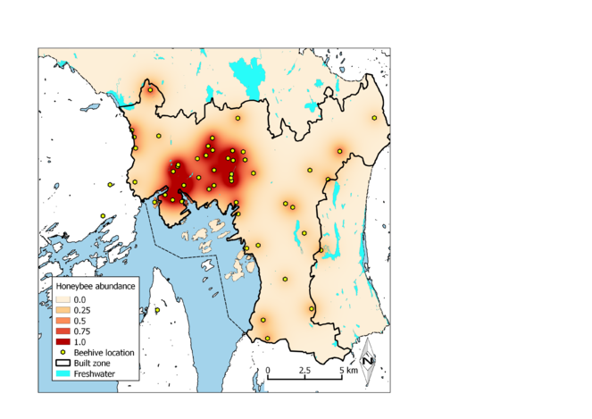
To model the distribution of domestic honeybees foraging in Oslo, we used the exact locations of permanent beehives provided to us by the ByBi beekeepers’ organisation and the number of hives per location. Honeybees—like all bee species—are central location foragers and travel only as far as necessary to collect food from flowers to minimise energy expenditure and mortality risk (
\(Honeybee foraging abundance=N*e^{(-0.002*D)}\),
where N = number of beehives at a given location and D = distance (m) from a given beehive location. We then divided the results of this expression by the maximum value so that all pixels scores ranged from 0 to 1. We subsequently identified regions within the municipality where foraging honeybees could have a comparatively greater potential to exhaust floral resources by subtracting ESTIMAP habitat suitability scores from foraging honeybee abundance scores. Pixels with values close to 1 indicate high honeybee to floral resource ratios, implying a greater potential for competition with wild bee species.
We used GRASS GIS 7.2.0 (
2.4 Field work for model validation
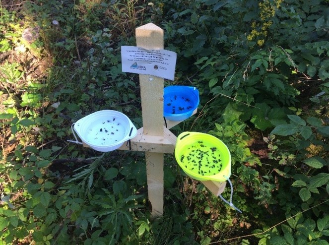
We collected pollinator specimens using pan traps, a common passive method used for sampling bees (
Results
The 74 trap dates yielded 2730 insects >4 mm long, with most insect captures (1933 individuals) belonging to the order Diptera (flies). Traps captured 395 individual bees—including 83 honeybees, 81 solitary bees and 231 bumblebees. Honeybee and solitary bee captures were highest for the July collection period (2.1 and 1.8 bees trap-1, respectively) while bumblebee captures were greatest in August (4.7 bees * trap-1). Total bee abundance (F1,72 = 4.93, P = 0.03), bee species richness (F1,72 = 5.16, P = 0.03), and bumblebee abundance F1,72 = 4.88, P = 0.03) all increased with increasing ESTIMAP habitat suitability scores for areas within a 50 m radius of trap locations (Supplementary material). Solitary bees' abundance (F1,72 = 0.39, P = 0.54) and species richness (F1,72 = 0.03, P = 0.95), and honeybee abundance (F1,72 = 2.83, P = 0.10) did not vary significantly with habitat suitability as expressed in the ESTIMAP model. The abundances of honeybees collected in traps did not vary significantly with the values from the foraging abundance model for the areas within either 50 (F1,72 = 0.29, P = 0.59) or 500 m (F1,72 = 0.28, P = 0.58) radii from trap locations. We found no evidence that greater numbers of honeybees were negatively associated with the abundance or species diversity of wild bees. Total bumblebee abundance (F1,73 = 9.64, P = 0.003), bumble species richness (F1,73 = 7.26, P = 0.01), solitary bee abundance (F1,73 = 8.34, P = 0.005) and solitary bee richness (F1,73 = 4.20, P = 0.04) corresponded positively with honeybee abundances.
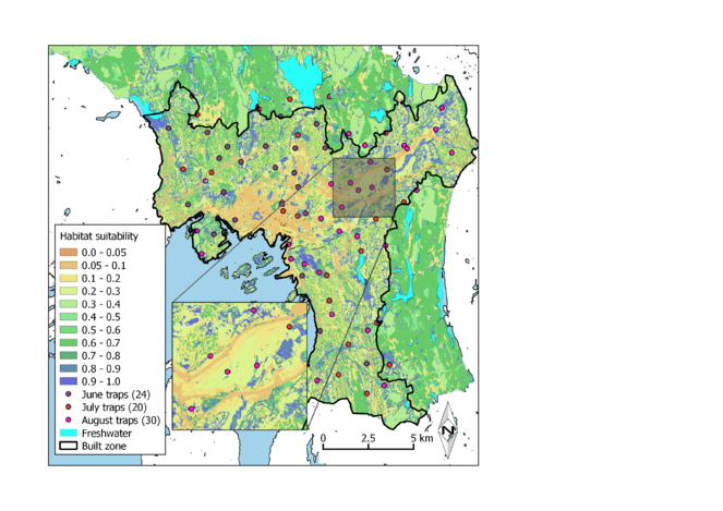
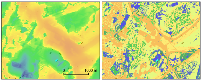
Our map of pollinator habitat suitability illustrates a considerable spatial heterogeneity within Oslo municipality (Fig.
Our model for foraging honeybee abundance (Fig.
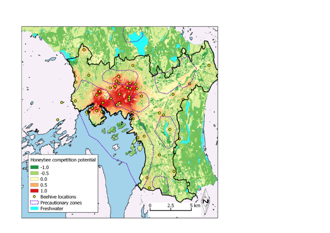
Map of the relative resource demand of foraging honeybees, accounting for the floral resource availability of the Oslo municipality landscape. Precautionary zones represent areas proposed by Oslo Urban Environmental Agency to protect potentially sensitive populations of red-listed wild bee species from competition with domestic honeybees.
Discussion
4.1 Modelling pollinator habitat suitability
The version of the model we present in Fig.
We also modified the original ESTIMAP model by eliminating the flight distance component, which is a change that we contend may be an appropriate approach for other models of pollinating insect abundances. We recognise the intuitive appeal with accounting for foraging flight in pollinator distribution models: bees are central place foragers and must bring food back to their nests to feed their offspring (
The Lonsdorf model performs reasonably well at the landscape scale in coarse grained or homogeneous landscapes (
The insect sampling which we conducted to validate our ESTIMAP model of bee habitat suitability confirms why models should not obscure the fine-grained spatial detail of floral resource distribution. Our traps’ captures generally reflected the habitat qualities of their immediate surroundings (within ≈ 50 metres) and corresponded less to trap sites’ larger landscape context. In other words, our trapping revealed high abundance and richness in small patches with ample flowers, even when these patches lay within larger areas dominated by low-suitability habitat. The Lonsdorf (
Investigations of urban bee communities underscore the important role that small, resource-rich patches play in supporting urban area’s wild bee populations (
4.2 Honeybee competition potential
Our empirical measures of bee abundance in Oslo provided no clear evidence of instances at trap sites where high numbers of honeybees appeared to displace wild bee species. In general, sites with greater numbers of honeybee also contained higher wild bee abundance and richness. Gunnarsson et al. (
Our work identified areas in Oslo where the impact of honeybee abundances is greatest relative to the distribution of floral resource availability (Fig.
Several recent studies employing manipulative experiments report evidence of competition between honeybees and wild bees, yet the details of the work suggest that the same dynamics may not be occurring in Oslo. Lindström et al. (
The honeybee addition treatments in Thomson (
The few examples of studies that explored competition between honeybees and solitary bees also failed to demonstrate clear evidence of negative effects of honeybees. Feral honeybees did not affect the reproductive success of a native Australian solitary bee (Megachile spp.), which the authors reasoned may be due to the native bee’s tolerance for extremely high summer temperatures (
4.3 Future research
The assessment we present here is admittedly incomplete as a means of determining the actual threat urban honeybees pose for the conservation of certain wild bee populations. We recommend two sampling approaches to further assess the vulnerability of wild bees in Oslo municipality. Figure 4 identifies the areas where competition from honeybees is most likely, and where future sampling efforts could be made more effective through concentrating on a smaller portion of the city's landscape. More focused insect trapping within these areas could reveal whether we actually see negative co-variation between honeybee and wild bee abundances that would indicate competition. We will conduct visual observations along transects at pan trap locations to verify data collected from pan traps and ensure that recorded observations include species that may not be susceptible to trapping. Visual observations will also allow us to assess the degree of resource overlap between honeybees and wild bees as demonstrated by which flowers different bee species are visiting. At the conservation priority sites that comprise the basis for precautionary zones, visual (non-destructive) assessment of bee abundance and resource use should also be conducted to estimate the intensity of honeybee foraging pressure at these sites.
The ESTIMAP model for Oslo can structure field surveys of urban vegetation according to the scores for habitat suitability (or floral availability). Information on the species identities of flowering plants, as well as the temporal availability (or phenology) of flowering resources, would serve as both a model validation and enhance the model’s capacity to describe distribution of biodiversity values within Oslo municipality. The Oslo Urban Environmental Agency has expressed an interest in this kind of information to help with urban planning, since it does not presently exist. Ideally, future vegetation surveys would include measurements of flower abundances and their variation through the growing season. Data on flowering plant communities’ species compositions, productivity and phenology would enable us to generate estimates of the landscape types’ supply of nectar and pollen. We could then compare floral resource supply with honeybees’ nutritional needs (per colony) and thereby assess the ecological footprint of urban beekeeping in Oslo. Modelling the appropriate honeybee stocking density for zoning purposes deserves further attention.
Another central research question that remains is how far do honeybees tend to fly from their hive locations, based on the distribution of floral resources in Oslo municipality. This information would determine the likelihood that honeybees will visit sites with conservation priority in abundances that would lead to competition with threatened wild bee species. Although we parameterised our model for honeybee abundance with empirical measurements of honeybee foraging, we readily acknowledge that our use of a simplistic diffusion-function may not be appropriate for the distribution of floral resources in Oslo and is worthy of the same criticisms we directed at the Lonsdorf and ESTIMAP continental-scale models. Using a CPF model based on our data on actual beehive locations, beehive numbers and the spatial patterns of suitable foraging habitat would most likely generate honeybee abundance predictions with greater spatial heterogeneity. However, both the Lonsdorf and the CPT models are highly sensitive to a parameter expressing the average distance a bee would travel. As we discussed earlier, bees’ average flight distance is not only a function of an individual’s physical capacity but also the actual need to seek food resources at greater distances from nest sites.
Fortunately, honeybees’ means of communicating foraging resource locations to other colony members via “waggle dances” provides us with a tool for estimating flight distances within a given landscape (
Research involving waggle dance decoding often involves assessing the type and amount of pollen found on the the legs of dancing bees, since this provides information about which flowers bees are utilising at a given site and whether the dancing bee is advertising sources or nectar or pollen (
4.4 Additional implications for management of urban biodiversity
One of the underlying goals of this study was to test the ability of the ESTIMAP model to express variation in the landscape that presumably determines variation in urban pollinator abundance and richness. Our empirical measurements from trap collections of the wild bee community partially predict the ESTIMAP habitat suitability output. Due to bees’ integral role in the reproduction of flowering plants, bees can function as indicator species for the status of the flowering plant community (
Bees’ ability to capitalise on small patches within the urban environment offer opportunities for small habitat improvement measures to yield large benefits (
Funding program
This work was funded by the European Union EU FP7 project OpenNESS (Grant agreement no. 308428) and URBAN SIS (Strategiske instituttsatsinger / SIS 2016-2019, Norwegian Research Council)
References
- Abrol DP (2012) Non bee pollinators-plant interaction. Pollination Biology.Springer,45pp.
- Bumble Bees (Bombus spp) along a Gradient of Increasing Urbanization.PLOS ONE4(5). https://doi.org/10.1371/journal.pone.0005574
- To Bee or Not to Bee.The Biologist60(4):12‑15.
- Where is the UK's pollinator biodiversity? The importance of urban areas for flower-visiting insects.Proceedings of the Royal Society B: Biological Sciences282(1803). https://doi.org/10.1098/rspb.2014.2849
- Using the waggle dance to determine the spatial ecology of honey bees during commercial crop pollination.Agricultural and Forest Entomology19:210‑216. https://doi.org/10.1111/afe.12204
- Wild bees along an urban gradient: winners and losers.Journal of Insect Conservation16(3):331‑343. https://doi.org/10.1007/s10841-011-9419-2
- Historical changes in northeastern US bee pollinators related to shared ecological traits.Proceedings of the National Academy of Sciences110(12):4656‑4660. https://doi.org/10.1073/pnas.1218503110
- EU FP7 OpenNESS Project Deliverable 33-44.European Commisson FP7
- (Dis)integrated valuation: narrowing the gap between ecosystem service appraisals and governance support.Ecosystem Services.
- Changing Bee and Hoverfly Pollinator Assemblages along an Urban-Rural Gradient.PLOS ONE6(8):e2345. https://doi.org/10.1371/journal.pone.0023459
- Long-range foraging by the honey-bee, Apis mellifera L.Functional Ecology14(4):490‑496. https://doi.org/10.1046/j.1365-2435.2000.00443.x
- Pollen DNA barcoding: current applications and future prospects 1.Genome59(9):629‑640. https://doi.org/10.1139/gen-2015-0200
- Butterflies in semi-natural pastures and power-line corridors – effects of flower richness, management, and structural vegetation characteristics.Insect Conservation and Diversity6(6):639‑657. https://doi.org/10.1111/icad.12019
- BIMBY’s first steps: a pilot study on the contribution of residential front-yards in Phoenix and Maastricht to biodiversity, ecosystem services and urban sustainability.Urban Ecosystems19(1):45‑76. https://doi.org/10.1007/s11252-015-0488-y
- Using citizen science to monitor pollination services.Ecological Entomology40:3‑11. https://doi.org/10.1111/een.12227
- Evaluating the effectiveness of wildflower seed mixes for boosting floral diversity and bumblebee and hoverfly abundance in urban areas.Insect Conservation and Diversity7(5):480‑484. https://doi.org/10.1111/icad.12071
- Ecological Impacts of Introduced Honey Bees.The Quarterly Review of Biology72(3):275‑297. https://doi.org/10.1086/419860
- Gauging the Effect of Honey Bee Pollen Collection on Native Bee Communities.Conservation Letters10(2):205‑210. https://doi.org/10.1111/conl.12263
- Complex Responses Within A Desert Bee Guild (Hymenoptera: Apiformes) To Urban Habitat Fragmentation.Ecological Applications16:632‑644. https://doi.org/10.1890/1051-0761(2006)016[0632:CRWADB]2.0.CO;2
- Effects of Suburbanization on Forest Bee Communities.Environmental Entomology43(2):253‑262. https://doi.org/10.1603/EN13078
- Landscape context and habitat type as drivers of bee diversity in European annual crops.Agriculture, Ecosystems & Environment133(1):40‑47. https://doi.org/10.1016/j.agee.2009.05.001
- Species richness declines and biotic homogenisation have slowed down for NW-European pollinators and plants.Ecology Letters16(7):870‑878. https://doi.org/10.1111/ele.12121
- Obligate association of an oligolectic bee and a seasonal aquatic herb in semi-arid north-eastern Brazil.Biological Journal of the Linnean Society102(2):355‑368. https://doi.org/10.1111/j.1095-8312.2010.01587.x
- Bumble bee species' responses to a targeted conservation measure depend on landscape context and habitat quality.Ecological Applications21(5):1760‑1771. https://doi.org/10.1890/10-0677.1
- Declines in forage availability for bumblebees at a national scale.Biological Conservation132(4):481‑489. https://doi.org/10.1016/j.biocon.2006.05.008
- Opinion: Why protect nature? Rethinking values and the environment.Proceedings of the National Academy of Sciences113(6):1462‑1465. https://doi.org/10.1073/pnas.1525002113
- Seasonal variation in pollen and nectar sources of honey bees in Ireland.Journal of Apicultural Research36(2):63‑76. https://doi.org/10.1080/00218839.1997.11100932
- Environmental consultancy: dancing bee bioindicators to evaluate landscape “health”.Frontiers in Ecology and Evolution3(44). https://doi.org/10.3389/fevo.2015.00044
- Waggle Dance Distances as Integrative Indicators of Seasonal Foraging Challenges.PLOS ONE9(4). https://doi.org/10.1371/journal.pone.0093495
- Honey bee foraging distance depends on month and forage type.Apidologie46(1):61‑70. https://doi.org/10.1007/s13592-014-0302-5
- Dancing Bees Communicate a Foraging Preference for Rural Lands in High-Level Agri-Environment Schemes.Current Biology24:1212‑1215.
- Intra-dance variation among waggle runs and the design of efficient protocols for honey bee dance decoding.Biology Open1(5):467‑472. https://doi.org/10.1242/bio.20121099
- Bees and beekeeping: science, practice and world resources.Heinemann Newnes,Oxford.
- Practical pollination ecology.Enviroquest Ltd,Cambridge, Ontario, Canada,590pp. [ISBN0968012307].
- Spanish rock art depicting honey gathering during the Mesolithic.Nature268(5617):228‑230. https://doi.org/10.1038/268228a0
- Pollination of lark daisy on roadsides declines as traffic speed increases along an Amazonian highway.Plant Biology18(3):542‑544. https://doi.org/10.1111/plb.12437
- Enhancing pollination supply in an urban ecosystem through landscape modifications.Landscape and Urban Planning162:157‑166. https://doi.org/10.1016/j.landurbplan.2017.02.011
- How much flower-rich habitat is enough for wild pollinators? Answering a key policy question with incomplete knowledge.Ecological Entomology40:22‑35. https://doi.org/10.1111/een.12226
- Land Cover 2000 (CLC2000) raster data—version 13 (02/2010).
- The Bee Fauna of Residential Gardens in a Suburb of New York City (Hymenoptera: Apoidea).Annals of the Entomological Society of America101(6):1067‑1077. https://doi.org/10.1603/0013-8746-101.6.1067
- Ecological Patterns of Bees and Their Host Ornamental Flowers in Two Northern California Cities.Journal of the Kansas Entomological Society78(3):227‑246. https://doi.org/10.2317/0407.08.1
- A DNA Barcoding Approach to Characterize Pollen Collected by Honeybees.PLOS ONE9(10):e109363. https://doi.org/10.1371/journal.pone.0109363
- Public approval plus more wildlife: twin benefits of reduced mowing of amenity grass in a suburban public park in Saltdean, UK.Insect Conservation and Diversity8(2):107‑119. https://doi.org/10.1111/icad.12085
- Eating locally: dance decoding demonstrates that urban honey bees in Brighton, UK, forage mainly in the surrounding urban area.Urban Ecosystems18(2):411‑418. https://doi.org/10.1007/s11252-014-0403-y
- Foraging ranges of solitary bees.Journal of Animal Ecology71(5):757‑764. https://doi.org/10.1046/j.1365-2656.2002.00641.x
- Diesel exhaust rapidly degrades floral odours used by honeybees.Scientific Reports3https://doi.org/10.1038/srep02779
- Combined effects of global change pressures on animal-mediated pollination.Trends in Ecology & Evolution28(9):524‑530. https://doi.org/10.1016/j.tree.2013.05.008
- Effects of Introduced Bees on Native Ecosystems.Annual Review of Ecology, Evolution, and Systematics34(1):1‑26. https://doi.org/10.1146/annurev.ecolsys.34.011802.132355
- Evidence for competition between honeybees and bumblebees; effects on bumblebee worker size.Journal of Insect Conservation13(2):177‑181. https://doi.org/10.1007/s10841-008-9140-y
- Decline and conservation of bumble bees.Annu Rev Entomol53:191‑208. https://doi.org/10.1146/annurev.ento.53.103106.093454
- Causes of rarity in bumblebees.Biological Conservation122(1):1‑8. https://doi.org/10.1016/j.biocon.2004.06.017
- Effects of land use at a landscape scale on bumblebee nest density and survival.Journal of Applied Ecology47(6):1207‑1215. https://doi.org/10.1111/j.1365-2664.2010.01872.x
- The impact of land use/land cover scale on modelling urban ecosystem services.Landscape Ecology31(7):1509‑1522. https://doi.org/10.1007/s10980-015-0337-7
- Geographic Resources Analysis Support System (GRASS) Software.Version 7.2.0..Open Source Geospatial Foundation.
- Bee foraging ranges and their relationship to body size.Oecologia153(3):589‑596. https://doi.org/10.1007/s00442-007-0752-9
- Bumblebees in the city: abundance, species richness and diversity in two urban habitats.Journal of Insect Conservation18(6):1185‑1191. https://doi.org/10.1007/s10841-014-9729-2
- The city as a refuge for insect pollinators.Conservation Biology31(1):24‑29. https://doi.org/10.1111/cobi.12840
- Norsk rødliste for arter 2015.Artsdatabanken, Norge.
- Competition between managed honeybees and wild bumblebees depends on landscape context.Basic and Applied Ecology17(7):609‑616. https://doi.org/10.1016/j.baae.2016.05.001
- Ecology of urban bees: a review of current knowledge and directions for future study.Cities and the Environment (CATE)2(1):article 3.
- Expansion of mass-flowering crops leads to transient pollinator dilution and reduced wild plant pollination.Proceedings of the Royal Society B: Biological Sciences278(1723):3444‑3451. https://doi.org/10.1098/rspb.2011.0268
- Competition between honey bees and wild bees and the role of nesting resources in a nature reserve.Journal of Insect Conservation17(6):1275‑1283. https://doi.org/10.1007/s10841-013-9609-1
- IPBES (2016) Chapter 5: Biocultural diversity, pollinators and their socio-cultural values. IPBES Thematic assessment of Pollinators, Pollination and Food Production.
- Aesthetic quality of agricultural landscape elements in different seasonal stages in Switzerland.Landscape and Urban Planning133:67‑77. https://doi.org/10.1016/j.landurbplan.2014.09.010
- Local resources, linear elements and mass-flowering crops determine bumblebee occurrences in moderately intensified farmlands.Agriculture, Ecosystems & Environment239:90‑100. https://doi.org/10.1016/j.agee.2016.12.039
- Techniques for pollination biologists.University Press of Colorado,Niwot, Colorado, USA.
- Endangered mutualisms: the conservation of plant-pollinator interactions.Annual review of ecology and systematics29(1):83‑112. https://doi.org/10.1146/annurev.ecolsys.29.1.83
- A global quantitative synthesis of local and landscape effects on wild bee pollinators in agroecosystems.Ecology Letters16(5):584‑599. https://doi.org/10.1111/ele.12082
- Pollinators as bioindicators of the state of the environment: species, activity and diversity.Agriculture, Ecosystems & Environment74(1–3):373‑393. https://doi.org/10.1016/S0167-8809(99)00044-4
- Importance of pollinators in changing landscapes for world crops.Proceedings of the Royal Society of London B: Biological Sciences274(1608):303‑313. https://doi.org/10.1098/rspb.2006.3721
- Lov om forvaltning av naturens mangfold (Naturmangfoldloven).
- Contrasting effects of mass-flowering crops on bee pollination of hedge plants at different spatial and temporal scales.Ecological Applications23(8):1938‑1946. https://doi.org/10.1890/12-2012.1
- Critical resource levels of pollen for the declining bee Andrena hattorfiana (Hymenoptera, Andrenidae).Biological Conservation134(3):405‑414. https://doi.org/10.1016/j.biocon.2006.08.030
- The Bee Inventory Plot.
- Pollinator Interactions with Yellow Starthistle (Centaurea solstitialis) across Urban, Agricultural, and Natural Landscapes.PLOS ONE9(1). https://doi.org/10.1371/journal.pone.0086357
- Light A (2006) Ecological citizenship: The democratic promise of restoration. In: RH P (Ed.) The Humane Metropolis: People and Nature in the 21st Century City.Univ of Massachusetts Press, Amherst, MA,Amherst, MA.
- Experimental evidence that honeybees depress wild insect densities in a flowering crop.Proceedings of the Royal Society B: Biological Sciences283(1843). https://doi.org/10.1098/rspb.2016.1641
- Modelling pollination services across agricultural landscapes.Annals of Botany103(9):1589‑1600. https://doi.org/10.1093/aob/mcp069
- Bumble bee abundance in New York City community gardens: implications for urban agriculture.Cities and the Environment (CATE)2(1).
- Direct and indirect effects of land use on floral resources and flower-visiting insects across an urban landscape.Oikos122(5):682‑694. https://doi.org/10.1111/j.1600-0706.2012.20229.x
- Buzz: Urban beekeeping and the power of the bee.NYU Press[ISBN1479874337]
- European Red List of Bees.Publication Office of theEuropean Union,Luxembourg. [ISBN978-92-79-44512-5] https://doi.org/10.2779/77003
- Norwegian Institute for Nature Researc.
- How many flowering plants are pollinated by animals?Oikos120(3):321‑326. https://doi.org/10.1111/j.1600-0706.2010.18644.x
- Modeling pollinating bee visitation rates in heterogeneous landscapes from foraging theory.Ecological Modelling316:133‑143. https://doi.org/10.1016/j.ecolmodel.2015.08.009
- Statistikkbanken. URL: http://statistikkbanken.oslo.kommune.no
- Impact of the introduced honey bee (Apis mellifera) (Hymenoptera: Apidae) on native bees: A review.Austral Ecology29(4):399‑407. https://doi.org/10.1111/j.1442-9993.2004.01376.x
- No short-term impact of honey bees on the reproductive success of an Australian native bee.Apidologie36(4):613‑621. https://doi.org/10.1051/apido:2005046
- Safeguarding pollinators and their values to human well-being.Nature540(7632):220‑229. https://doi.org/10.1038/nature20588
- Role of nesting resources in organising diverse bee communities in a Mediterranean landscape.Ecological Entomology30(1):78‑85. https://doi.org/10.1111/j.0307-6946.2005.00662.x
- Declines of managed honey bees and beekeepers in Europe.Journal of Apicultural Research49(1):15‑22. https://doi.org/10.3896/IBRA.1.49.1.02
- Team,2017QGIS 2.18.6 (Las Palmas).
- Widespread exploitation of the honeybee by early Neolithic farmers.Nature534(7607):1‑2. https://doi.org/10.1038/nature18451
- The role of resources and risks in regulating wild bee populations.Annu Rev Entomol56:293‑312. https://doi.org/10.1146/annurev-ento-120709-144802
- RStudio: Integrated Development for R.RStudio, Inc., Boston, MA.
- Urban habitats for bees: the example of the city of Berlin.18.Linnean Society Symposium Series.ACADEMIC PRESS LIMITED,7pp. [ISBN0161-6366].
- Pollination of Campanula rapunculus L. (Campanulaceae): How much pollen flows into pollination and into reproduction of oligolectic pollinators?Plant Systematics and Evolution250:147‑156. https://doi.org/10.1007/s00606-004-0246-8
- Lessons learned for spatial modelling of ecosystem services in support of ecosystem accounting.Ecosystem Services13:64‑69. https://doi.org/10.1016/j.ecoser.2014.07.003
- The wisdom of the hive : the social physiology of honey bee colonies.Harvard University Press,Cambridge, Massachusetts. [ISBNISBN 0-674-95376-2]
- Honey bee foragers as sensory units of their colonies.Behavioral Ecology and Sociobiology34(1):51‑62. https://doi.org/10.1007/bf00175458
- Adding ecological value to the urban lawnscape. Insect abundance and diversity in grass-free lawns.Biodiversity and Conservation24(1):47‑62. https://doi.org/10.1007/s10531-014-0788-1
- Do resources or natural enemies drive bee population dynamics in fragmented habitats.Ecology89(5):1375‑1387. https://doi.org/10.1890/06-1323.1
- Scale-dependent effects of landscape context on three pollinator guilds.Ecology83(5):1421‑1432. https://doi.org/10.2307/3071954
- MultiNet® Shapefile Format Specification.
- Competitive interactions between the invasive European honey bee and native bumble bees.Ecology85(2):458‑470. https://doi.org/10.1890/02-0626
- Bee diversity and abundance in an urban setting.Canadian Entomologist136(6):851‑869. https://doi.org/10.4039/n04-010
- Collateral effects of beekeeping: Impacts on pollen-nectar resources and wild bee communities.Basic and Applied Ecology17(3):199‑209. https://doi.org/10.1016/j.baae.2015.11.004
- Determinants of Spatial Distribution in a Bee Community: Nesting Resources, Flower Resources, and Body Size.PLOS ONE9(5). https://doi.org/10.1371/journal.pone.0097255
- Intangible Cultural Heritage Section, Division for Creativity, Culture Sector.Paris,132pp.
- World Population Prospects: The 2015 Revision, Volume I: Comprehensive Tables. ST/ESA/SER.A/379.ST/ESA/SER.A/379..United Nations Department of Economic and Social Affairs, Population Division.
- Threats to an ecosystem service: pressures on pollinators.Frontiers in Ecology and the Environment11(5):251‑259. https://doi.org/10.1890/120126
- Foraging Strategy of Honeybee Colonies in a Temperate Deciduous Forest.Ecology63(6):1790‑1801. https://doi.org/10.2307/1940121
- The dance language and orientation of bees.Harvard University Press,Cambridge.
- Foraging distances of Bombus muscorum, Bombus lapidarius, and Bombus terrestris (Hymenoptera, Apidae).Journal of Insect Behavior13(2):239‑246. https://doi.org/10.1023/A:1007740315207
- Increased density of honeybee colonies affects foraging bumblebees.Apidologie37(5):517‑532. https://doi.org/10.1051/apido:2006035
- Measuring bee diversity in different European habitats and biogeographical regions.Ecological monographs78(4):653‑671. https://doi.org/10.1890/07-1292.1
- Westrich P (1996) Habitat requirements of central European bees and the problems of partial habitats. In: Matheson A, Buchmann SL, O'Toole WP, Williams IH (Eds) The Conservation of Bees.Academic Press,London.
- The conservation and restoration of wild bees.Annals of the New York Academy of Sciences1195(1):169‑197. https://doi.org/10.1111/j.1749-6632.2010.05449.x
- Effect of Human Disturbance on Bee Communities in a Forested Ecosystem.Conservation Biology21(1):213‑223. https://doi.org/10.1111/j.1523-1739.2006.00574.x
- Enhancing floral resources for pollinators in productive agricultural grasslands.Biological Conservation171:44‑51. https://doi.org/10.1016/j.biocon.2014.01.023
- Pollinator habitat enhancement: Benefits to other ecosystem services.Agriculture, Ecosystems & Environment159:112‑122. https://doi.org/10.1016/j.agee.2012.06.020
- Effects of urbanization on Neotropical wasp and bee assemblages in a Brazilian metropolis.Landscape and Urban Planning71:105‑121. https://doi.org/10.1016/j.landurbplan.2004.02.003
- Linking Land Cover Data and Crop Yields for Mapping and Assessment of Pollination Services in Europe.Land2(3):472‑492. URL: http://www.mdpi.com/2073-445X/2/3/472